Understanding differences in applying DETR to natural and medical images

Xu, Yanqi; Shen, Yiqiu; Fernandez-Granda, Carlos; Heacock, Laura; Geras, Krzysztof J.

doi:https://doi.org/10.59275/j.melba.2025-g137

1 Introduction

Refer to caption — Figure 1: An overview of the study. In this work, we investigate key design choices in Deformable DETR using the NYU Breast Cancer Screening Dataset (NYU Breast) and LUNA16 Dataset. Specifically, we evaluate six design factors (highlighted in red): (1) input resolution, (2) number of encoder layers, (3) use of multi-layer feature fusion, (4) number of object queries, (5) query initialization method, and (6) use of iterative bounding box refinement. The graph on the right shows changes in Average Precision (AP) resulting from these design choices. +2 indicates a reduction in encoder layers; +3 removes multi-layer fusion; +4 reduces object queries; +5 adds query initialization; and +6 enables iterative box refinement. Our findings suggest that a simplified architecture (+2,3,4) is better suited for medical datasets, leading to improved performance.

Recent advances in computer vision have increasingly turned to transformer architectures (Vaswani et al., 2017) for tasks such as image classification and object detection (Dosovitskiy et al., 2020; Liu et al., 2021; Carion et al., 2020; Touvron et al., 2021). With their inherent self-attention mechanisms, transformers effectively capture global dependencies and understand contextual relations across the entire image. These strengths have made transformer-based models a popular choice in natural image analysis. Their application in medical imaging has shown promising results, suggesting strong potential in this field as well (Chen et al., 2021; Dai et al., 2021b; Valanarasu et al., 2021; Zheng et al., 2022).

Object detection is crucial in medical image analysis, as detection models identify the locations of abnormalities, which are important for medical diagnosis. Among transformer-based detectors, Detection Transformer (DETR) (Carion et al., 2020) has gained popularity for its end-to-end training pipeline and elimination of non-differentiable post-processing steps such as Non-Maximum Suppression (NMS) (Girshick et al., 2014). By leveraging the transformer architecture and directly optimizing the objective function, DETR achieves state-of-the-art results on natural image benchmarks such as MS COCO (Zhu et al., 2020; Zhang et al., 2022; Zong et al., 2023). Its success has drawn intense research interest, leading to a range of highly engineered DETR variants aimed at boosting accuracy and training efficiency (Zhu et al., 2020; Zhang et al., 2022; Chen et al., 2022b; Wang et al., 2022; Chen et al., 2022a).

Despite the success of DETR architectures on natural image benchmarks, their direct application to medical imaging remains challenging due to fundamental differences between the two domains (Figure 2):

•
High resolution and small regions of interest: Medical images are often extremely high-resolution, with clinically relevant features, such as lesions or calcifications, occupying only small portions of the image (Moawad et al., 2023; Heath et al., 2001).
•
Standardized acquisition protocols: Unlike natural images which have diverse backgrounds, medical images are acquired under standardized procedures, resulting in consistent anatomical structures and minimal background variability.
•
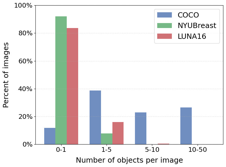
Few objects per image: Medical images usually focus on a narrow range of abnormalities, resulting in fewer objects of interest and a narrower class space compared to the rich and diverse class space of natural images. Additionally, many medical images may not contain any objects at all.
•
Small and imbalanced data sets: Medical imaging data sets are often small and exhibit a more unbalanced class distribution, as positive cases (i.e., unhealthy subjects) are usually much less common than negative cases (i.e., healthy subjects)(Galdran et al., 2021; Heath et al., 2001; Wang et al., 2017).

DETR-family models, such as Deformable DETR (Zhu et al., 2020), incorporate complex design choices such as multi-scale feature fusion and iterative bounding box refinement to address challenges in natural image detection. However, their effectiveness in medical imaging is unclear, as the domain presents distinct characteristics: high resolution, small lesion size, limited object diversity, and class imbalance, which differ markedly from natural images. In such settings, detecting subtle features precisely is often more important than modeling diverse object scales or dense scenes. As a result, these complex design choices may introduce unnecessary computational overhead and memory cost without yielding performance gains.

In this study, we examine how DETR can be adapted to better suit medical imaging tasks. We hypothesize that a simplified model, tailored to the specific characteristics of medical data, can achieve comparable performance with reduced computational cost. To evaluate this, we use Deformable DETR (Zhu et al., 2020) as a baseline on two medical imaging datasets: the NYU Breast Cancer Screening Dataset (Wu et al., 2019) and the LUNA16 dataset (Setio et al., 2017), a public chest CT dataset focused on lung nodule detection (Figure 2). Those two datasets highlight the distinct features of medical images, such as high resolution, small lesions, and class imbalance.

Our experiments demonstrate that simplified DETR configurations—using fewer encoder layers, a single feature map, and no decoding enhancements—achieve detection performance on par with, or better than, standard Deformable DETR, while substantially reducing computational cost. These findings validate our hypothesis and highlight the potential of lightweight DETR variants as efficient and effective baselines for medical imaging. The key findings of our work are:

•
Models with a reduced number of encoder layers and no multi-scale feature fusion learn faster without compromising detection performance. These changes maintain performance within $1\%$ in $\mathrm{AP}_{10,50}$ on both datasets, while accelerating training by up to 40%.
•
Increasing the number of object queries to around 100 queries improves localization and detection performance. Beyond this point, performance declines, primarily due to a rise in false positives that obscure true positive detections.
•
Decoding techniques such as object query initialization and iterative bounding box refinement, while beneficial for natural image detection, do not improve performance on medical datasets. In some cases, they degrade performance (e.g., a 0.7% drop in $\mathrm{AP}_{10,50}$ for NYU Breast and 1.8% drop for LUNA16), likely due to overfitting and limited positive examples.

2 Background on DETRs

DETR (Carion et al., 2020) offers several advantages over traditional detection models such as Mask-RCNN (He et al., 2017) and YOLO (Redmon et al., 2016). Its transformer-based architecture enables more expressive feature representations, and its end-to-end training simplifies optimization and improves performance. However, DETR suffers from slow learning. To address this issue, various extensions have been proposed to accelerate training and improve detection performance (Zhu et al., 2020; Wang et al., 2022; Chen et al., 2022b; Zhang et al., 2022). Deformable DETR (Zhu et al., 2020) stands out for its competitive performance on the MS COCO dataset (Lin et al., 2014). It introduces a deformable attention module that reduces training time by a factor of 10 and enables multi-scale feature fusion that improves detection, especially for small objects. Given its strong performance and widespread adoption in subsequent research (Roh et al., 2021; Dai et al., 2021a; Zhang et al., 2022; Yao et al., 2021), we adopt Deformable DETR as the baseline for our experiments. This section outlines the key components of DETR and Deformable DETR architectures.

DETR

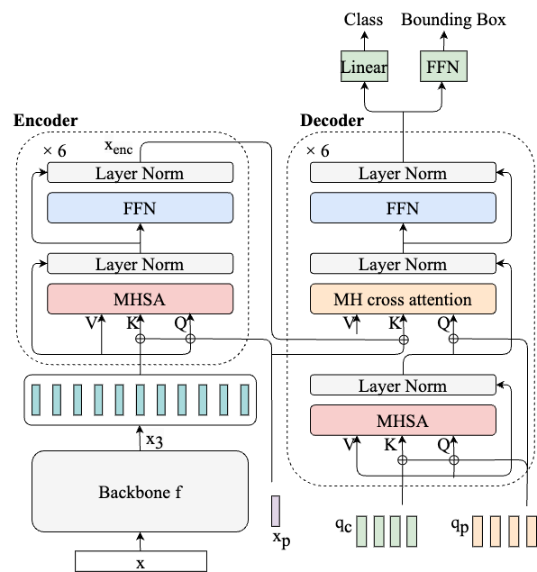
DETR (Carion et al., 2020) consists of a backbone, an encoder-decoder transformer, and a prediction head, as illustrated in Figure 3(a).

Given an input image $x\in\mathbb{R}^{C_{0}\times W_{0}\times H_{0}}$ , where $C_{0}$ is the number of channels and $W_{0}$ and $H_{0}$ are the width and height, the backbone network $f$ produces a low-resolution activation map $x_{s}=f(x)\in\mathbb{R}^{C\times W\times H}$ , with $C$ significantly larger than $C_{0}$ . The specific sizes of $W,H$ and $C$ depend on the choice of backbones. For instance, when using Swin-T (Liu et al., 2021) as the backbone, the spatial dimensions are downsampled to $W=W_{0}/32$ and $H=H_{0}32$ , and the number of channels is increased to $C=768$ . This map is further processed by a $1\times 1$ convolution to collapse the channel dimension $C$ into a smaller size $d$ , resulting in image tokens $x_{f}=\mathrm{conv}(x_{s})\in\mathbb{R}^{WH\times d}$ . To preserve spatial information in the original image, each token is paired with a positional encoding, denoted by $x_{p}\in\mathbb{R}^{WH\times d}$ . The encoder is a standard attention-based transformer where each layer consists of a multi-head self-attention module (MHSA) followed by a feedforward network (FFN). For an in-depth formalization of MHSA, refer to the Appendix A.1. Typically, the DETR encoder consists of 6 layers. The encoder preserves the dimension of the input, producing $x_{enc}\in\mathbb{R}^{WH\times d}$ .

The decoder receives two inputs, the encoded features $x_{enc}$ and $N$ object queries $q\in\mathbb{R}^{N\times d}$ . Object queries play a central role in the DETR architecture. They are learnable embeddings that work as placeholders for potential objects in an image. Each of them attends to the specific regions of the image and is individually decoded into a bounding box prediction. Each object query is the sum of two learnable embeddings: content embeddings $q_{c}\in\mathbb{R}^{N\times d}$ , initialized as zero vectors, and positional embeddings $q_{p}\in\mathbb{R}^{N\times d}$ , indicating each query’s position. More methods for initializing object queries are discussed in Section 3. Decoder layers consists of a MHSA, enabling inter-query learning, and multi-head (MH) cross-attention to integrate encoder features, and an FFN. The formalization of MH cross-attention is detailed in the Appendix A.2.

After the decoder, each object query is independently decoded into bounding box coordinates and class scores through a three-layer FFN and a linear layer respectively.

Deformable DETR

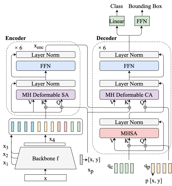
Deformable DETR (Zhu et al., 2020) improves upon DETR by introducing a deformable attention module, which accelerates training and enhances the detection of small objects. The architecture of Deformable DETR is illustrated in Figure 3(b).

Unlike the standard attention mechanism that calculates attention scores between all query-key pairs, resulting in $(WH)^{2}$ pairs for a feature map of size $W\times H$ , deformable attention selectively computes attention scores on a subset of $k<<WH$ keys for each query. The subset is selected through a learnable key sampling function, allowing the model to focus on the most informative regions for each query. For a detailed formalization of the deformable attention module, refer to Appendix B.1.

For dense prediction tasks such as object detection, incorporating higher-resolution feature maps can substantially improve detection performance, especially for smaller objects (He et al., 2017). However, the complexity of the standard attention mechanism is quadratic with respect to the number of tokens, making it infeasible for multiple scales of feature maps. The deformable attention mechanism enables effective multi-scale feature fusion. Specifically, the encoder receives the output feature maps $x_{1},x_{2},x_{3}$ from the last three layers of the backbone, and a convolutional layer generates the lowest resolution feature map $x_{4}$ . All four feature maps undergo a $1\times 1$ convolution and then are reshaped into a sequence of feature vectors of dimension $d$ , denoted by $x_{f}\in\mathbb{R}^{M\times d}$ . Each token is associated with a positional embedding, as well as a layer embedding to identify feature map level. Section 3 explores the benefits of multi-feature fusion for medical imaging datasets.

Moreover, Deformable DETR introduces reference points in the deformable attention module. In the encoder, each query $q$ is associated with a 2D reference point $p_{q}=[x,y]$ , denoting its location on the feature map. The key sampling function generates $k$ sampling offsets with respect to the reference point, and thus determines the $k$ keys for the query. Similarly in the decoder, the reference point of each object query $q$ is defined by a linear projection of its positional embedding $q_{p}$ . In this way, each object query can be mapped to a position on the feature map. This approach allows object queries to focus on specific regions, significantly accelerating learning (Zhu et al., 2020).

DETR in Medical Imaging

DETR-based architectures have been widely applied to various medical imaging tasks, often with architectural tweaks to improve overall performance. For example, Mathai et al. (2022) leveraged a bounding box fusion technique in DETR to reduce the false positive rate in lymph nodes detection. MyopiaDETR (Li et al., 2023) utilizes a Feature Pyramid Network to improve the detection of small objects in lesion detection of pathological myopia. COTR (Shen et al., 2021) embeds convolutional layers into DETR encoders to accelerate learning in polyp detection. Although these works achieved good performances, our experiments indicate that, contrary to the common understanding, simplifying the DETR architecture can improve accuracy and accelerate training. We identified a work that also points in this direction, Cell-DETR (Prangemeier et al., 2020), also reduces the number of parameters tenfold, achieving faster inference speeds while maintaining performance on par with state-of-the-art baselines. Finally, Garrucho et al. (2023) applied out-of-the-box Deformable DETR on mammography for mass detection. However, their focus is the effect of a data augmentation method on its detection performance. Despite these advances, a systematic exploration of the effectiveness and relevance of foundational DETR design choices remains underexplored.

3 Methods

3.1 Design Choices

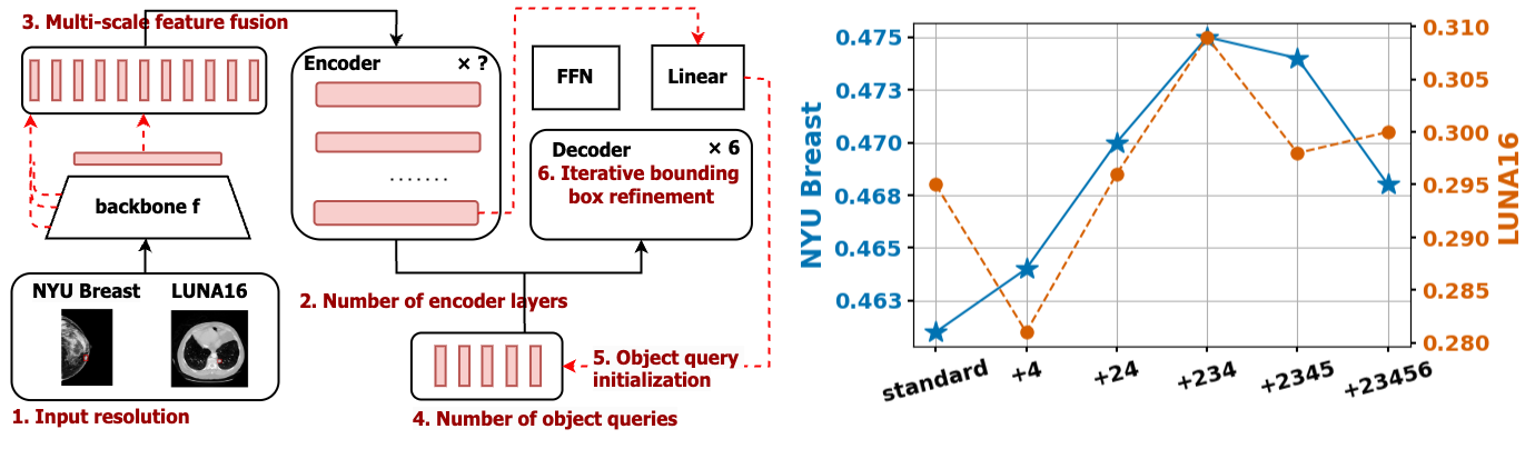
In this section, we outline key design choices in Deformable DETR that are relevant to the unique characteristics of medical images: input resolution, the number of encoder layers, multi-scale feature fusion, the number of object queries, and two techniques enhancing the decoding process, query initialization and iterative bounding box refinement (IBBR). We investigated whether these components, which improve performance on natural image datasets, offer similar benefits when applied to medical imaging tasks.

Input resolutions

Downsampling is commonly used in detection models to reduce computational cost and satisfy memory constraints. Natural images can be significantly downsized to $224\times 224$ or $256\times 256$ pixels without losing important features, such as edges, shapes, and textures that are necessary for accurate predictions. In contrast, medical images are often an order of magnitude larger. For example, X-ray images can reach up to $2500\times 3056$ pixels (Johnson et al., 2019), and CT scans are typically $512\times 512$ pixels (Setio et al., 2017). These high-resolution medical images contain fine-grained details, such as small lesions or slight changes in tissue density, which are crucial for an accurate diagnosis (Sabottke and Spieler, 2020; Thambawita et al., 2021). However, processing high-resolution medical images is often infeasible due to the high computational requirements. To address this trade-off, we evaluate performance across input resolutions ranging from 25% to 100% of the original size, aiming to identify the optimal input resolution that balances model accuracy with computational efficiency and memory usage.

Encoder complexity

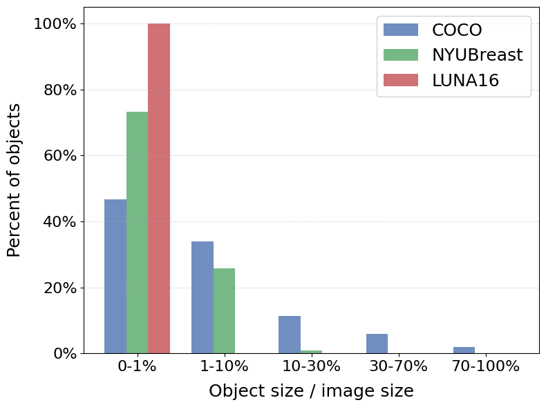
Medical imaging datasets differ from natural image datasets in several important ways. First, they are typically smaller due to limited patient availability. Second, images within a dataset tend to be homogeneous, focusing on a single body part, such as the brain, breast, or chest, with uniform grayscale textures (Figure 2). Third, while natural images contain hundreds or thousands of object classes, medical image datasets usually have far fewer object classes. For example, NIH Chest X-ray contains 14 classes (Wang et al., 2017), DDSM has 2 (Heath et al., 2001), and BraTS has 4 (Moawad et al., 2023). As a result, there is much less variation in the data that the model has to capture. Given the principle that model complexity should align with task complexity (Geman et al., 1992), we suspect that simpler, shallower architectures might be more appropriate for medical image analysis, helping mitigate overfitting and improve training efficiency. In addition, object sizes in medical images are typically more uniform than in natural scenes. For example, the standard deviation of normalized object sizes¹¹1Normalized object size refers to the area of the bounding box divided by the total image area. is 0.025 in the NYU Breast Cancer Screening Dataset and 0.001 in LUNA16, compared to 0.16 in MS COCO. This raises questions about the use of multi-scale feature fusion in this domain, a technique primarily intended to improve detection across diverse object sizes. To investigate these hypotheses, we experimented with modifications to the encoder of Deformable DETR, including reducing the number of encoder layers and utilizing fewer scales of feature maps from the backbone.

Number of object queries

In DETR, each object query is individually decoded into a bounding box prediction. Thus, the total number of object queries determines how many objects the model can detect per image (Carion et al., 2020). Most DETR models are optimized for natural image datasets such as MS COCO, where a single image can contain up to $100$ objects. Consequently, the number of object queries is usually set to $300$ in DETR models. In contrast, medical images rarely contain more than 10 objects, and most have only one or none. As a result, the default number of object queries used in standard DETR implementations may be excessive for medical applications, potentially leading to unnecessary computation or degraded performance. We therefore examine how reducing the number of object queries affects detection accuracy and efficiency on medical image datasets.

Decoding techniques

Many DETR variants apply object queries initialization and iterative bounding box refinement (IBBR) to improve query decoding and increase detection accuracy (Zhu et al., 2020; Zhang et al., 2022; Yao et al., 2021). These methods have proven effective in boosting detection performance on natural image datasets, increasing average precision by 2.4 on the MS COCO dataset (Zhu et al., 2020). In this study, we evaluate their effectiveness in the medical imaging domain. We tested three initialization strategies for the positional and content embeddings of object queries, as characterized by Zhang et al. (2022).

•
Static queries Both positional and content embeddings are randomly initialized as learnable embeddings. This offers maximum flexibility, but requires the model to learn where objects are likely located and what features represent those objects from scratch, potentially slowing convergence. Standard Deformable DETR uses this approach.
•
Pure query selection Both content and positional embeddings are initialized from selected encoder features. Following Zhu et al. (2020), we apply the prediction head to the encoder output to select the top- $K$ features. Some other works use a regional proposal network (Yao et al., 2021; Chen et al., 2022b). This leverages encoder knowledge to guide object queries and significantly accelerates training.
•
Mixed Query Selection: Positional embeddings are initialized from encoder features (as above), while content embeddings remain randomly initialized. This hybrid strategy informs about the likely positions of objects through spatial priors while retaining flexibility in learning content representations from scratch. DETR with Improved DeNoising Anchor Boxes (DINO) (Zhang et al., 2022) found that this method yields the best performance.

IBBR, first introduced in Deformable DETR, iteratively updates the reference points of object queries towards the objects of interest in each image. These reference points guide the deformable attention toward relevant regions to search for objects. Initially, they are randomly distributed across the image, ensuring broad coverage without any prior knowledge about where objects might be located. With IBBR, these reference points can move progressively towards the objects through each decoder layer, providing more accurate signals for attention. This technique has been extensively applied in subsequent DETR variants (Zhu et al., 2020; Chen et al., 2022b; Wang et al., 2022; Liu et al., 2022) and has been shown to effectively speed up training and improve detection performance. A detailed formalization is provided in the Appendix C.

3.2 Data and task

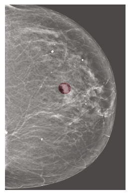
NYU Breast Cancer Screening Dataset (NYU Breast)

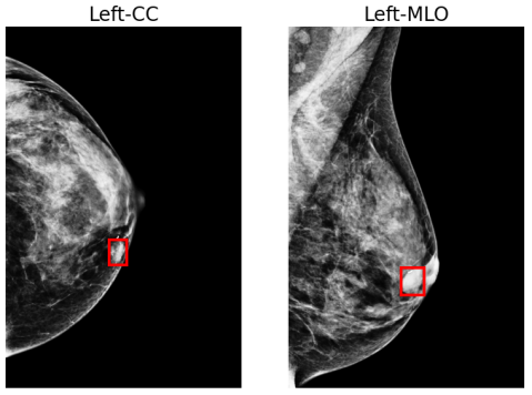
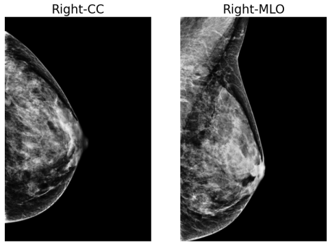
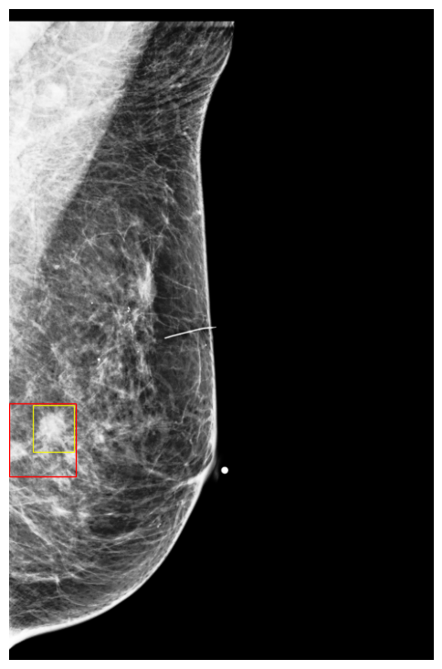
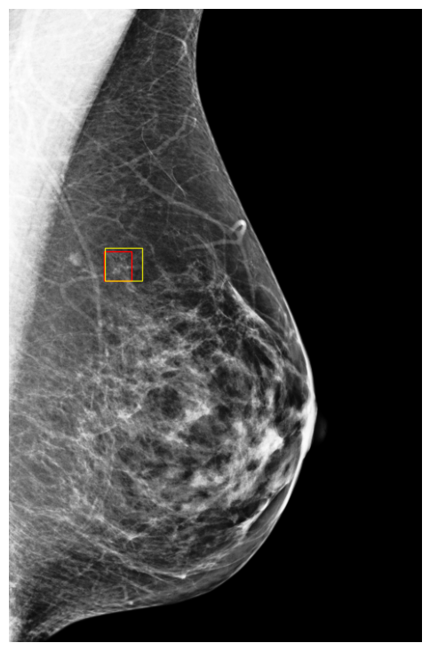
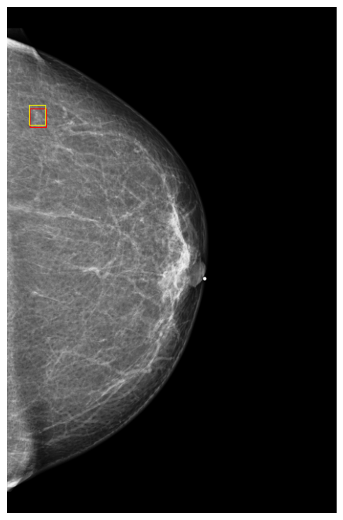
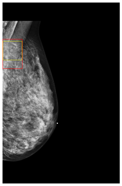
(Wu et al., 2019) contains $229,426$ digital screening mammography exams from $141,472$ patients screened at NYU Langone Health. Each exam includes a minimum of four images, each with a resolution of $2944\times 1920$ , covering two standard screening views: craniocaudal (CC) and mediolateral oblique (MLO), for both the left and right breasts. An example of a mammography exam is shown in Figure 4. The dataset is annotated with breast-level cancer labels indicating biopsy-confirmed benign or malignant findings. Moreover, the dataset also provides bounding box annotations, and class labels (benign or malignant) of each visible positive findings. The entire dataset contains $985$ breasts with malignant findings and $5,556$ breasts with benign findings. The dataset is divided into training ( $82\%$ ), validation ( $5\%$ ) and test sets ( $13\%$ ) ensuring a proportional distribution of benign and malignant cases across the subsets.

LUNA16

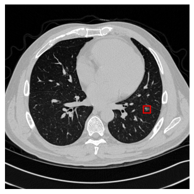
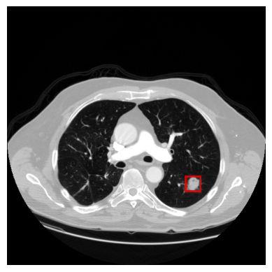
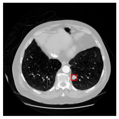
LUNA16 (Setio et al., 2017) is a public chest CT dataset for lung nodule detection, containing 888 3D chest CT scans with annotated nodule locations. We selected this dataset because it exemplifies key characteristics of medical imaging (Figure 5): (1) high resolution (typically 512 x 512 pixels per slice), necessary for capturing fine details; (2) small objects of interest, as nodules are subtle and occupy only a small portion of each scan; and (3) class imbalance, as nodules are relatively rare. Each nodule is annotated in 3D with a center point $(x,y,z)$ and diameter. To convert them into 2D bounding boxes, we identify the slices intersecting each nodule along the z-coordinate and project the center point to 2D $(x,y)$ coordinates on each slice. Using the diameter, we define a 2D bounding box around this point, allowing slice-by-slice nodule detection. Since DETR is designed for 2D object detection, we treat each 2D slice as an independent input to the model, enabling nodule detection in each slice separately. The dataset is randomly split for training (666 scans, 75%), validation (88 scans, 10%), and test (134 scans, 15%).

3.3 Evaluation Metrics

In this study, we focus on evaluating the ability of the models to detect malignant lesions. We use Average Precision (AP) (Everingham et al., 2010) and the Free-Response Receiver Operating Characteristic curve area (FAUC) (Bandos et al., 2009), which is a frequently used metric in medical image analysis (Yu et al., 2022; Wang et al., 2018; Petrick et al., 2013). Specifically, we focus on FAUC at the rate of 1 false positive per image or smaller, referred to as $\mathrm{FAUC}^{1}$ , in line with the approach described by Bandos et al. (2009). To formalize $\mathrm{FAUC}^{1}$ , we introduce the following notation:

Let N denote the total number of images, indexed by $n=1,2,..,N$ . Each image $n$ contains $L_{n}$ lesions with $L_{total}=\sum^{N}_{1}L_{n}$ being the total lesions in the dataset. For each image $n$ , a detection model produces a set of candidate detections $\mathcal{D}_{n}=\{d_{n}^{1},d_{n}^{2},...\}$ , each with a confidence score $s(d_{n}^{j})$ . By varying a decision threshold $\tau$ , one can include only those detections whose scores exceed $\tau$ , denoted $\mathcal{D}_{n}(\tau)=\{d\in\mathcal{D}_{n}:s(d)\leq\tau\}$ .

Following prior works (Jailin et al., 2023; Kolchev et al., 2022; Konz et al., 2023), we define a positive bounding box to have at least 10% Intersection over Union (IoU) with a ground truth box. These thresholds are deemed more appropriate for accurately detecting small-sized objects, such as cancerous lesions. The $\mathrm{FAUC}^{1}_{10}$ metric integrates the true positive rate (TPR) over false positives per image (FPI) from 0 to 1:

\mathrm{FAUC}^{1}_{10}=\int^{1}_{0}\frac{1}{L_{total}}\sum^{n}_{n=1}\sum^{L_{n}}_{m=1}1(\exists d\in\mathcal{D}_{n}(\tau(u)):d\leftrightarrow L_{n}^{m})du,

where:

•
$\tau(u)$ is the threshold achieving $\mathrm{FPI}=\frac{1}{N}\sum_{N=1}^{N}|\{d\in\mathcal{D}_{n}(\tau):d\nleftrightarrow L_{n}^{m},\forall m\in L_{n}\}=u$
•
$d\leftrightarrow L_{n}^{m}$ indicates the lesion $m$ is detected by the prediction $d$ in image $n$

Following the notation of integrated average precision in PASCAL VOC 2012 (Salton, 1983; Everingham et al., 2010), we denote AP at 0.1 IoU threshold as $\mathrm{AP}_{10}$ . Additionally, we report the average AP across IoU thresholds ranging from 0.1 to 0.5, in steps size of 0.05, denoted as $\mathrm{AP}_{10,50}$ .

To clearly explain how well our models detect objects, we differentiate between “localization” and “classification.”

•

Localization refers to the task of accurately drawing a bounding box around each ground-truth object. To be consistent with the definition of FAUC and AP, an object is considered successfully localized if the model produces a bounding box overlapping the ground truth box by more than 10% IoU. To quantify localization accuracy, we compute the percentage of ground-truth objects successfully detected by the model. Assume there are $m$ ground-truth objects $G_{i}$ where $i=1,\ldots,m$ and $p$ predicted boxes $P_{j}$ where $j=1,\ldots,p$ in an image. The maximum IoU for a ground truth bound box $G_{i}$ among all predicted bounding boxes $P_{j}$ is $\max_{j}(\mathrm{IoU}(P_{j},G_{i}))$ . Localization accuracy $L$ is then expressed as

L=\frac{1}{m}\sum^{m}_{i=1}\mathds{1}_{\max_{j}\left({\mathrm{IoU}\left(P_{j},G_{i}\right)}\right)\geq 0.1},

(1)

where the indicator function is defined as

\mathds{1}_{\max_{j}\left({\mathrm{IoU}\left(P_{j},G_{i}\right)}\right)\geq 0.1}=\begin{cases}1,&\mathrm{if}\max_{j}\left(\mathrm{IoU}\left(P_{j},G_{i}\right)\right)\geq 0.1\\ 0,&\mathrm{otherwise}.\end{cases}

•

Classification involves associating the object inside each predicted box with the correct class. We consider models’ classification accuracy using the percentage of successfully localized objects among the predicted bounding boxes with the top 10 highest predicted scores in each image. Among all the predicted bounding boxes $P_{j}$ in an image, let $S$ be the subset of indices of the top 10 predicted bounding boxes in an image. Localization performance considering classification is expressed as

L_{\mathrm{top10}}=\frac{1}{m}\sum^{m}_{i=1}\mathds{1}_{\max_{j\in S}({\mathrm{IoU}(P_{j},G_{i})})\geq 0.1},

(2)

where the indicator function is defined as

	$\displaystyle\mathds{1}_{\max_{j\in S}\left({\mathrm{IoU}\left(P_{j},G_{i}\right)}\right)\geq 0.1}$	$\displaystyle=$
		$\displaystyle\begin{cases}1,&\mathrm{if}\max_{j\in S}\left(\mathrm{IoU}\left(P_{j},G_{i}\right)\right)\geq 0.1\\ 0,&\mathrm{otherwise}.\end{cases}$

3.4 Experimental Setup

Our baseline model is Deformable DETR in its default setting, using a Swin-T backbone (Liu et al., 2021). For the NYU Breast Cancer Screening dataset, the backbone is pretrained on a breast cancer classification task using the same dataset (see Appendix D for details). Models are trained for 60 epochs on NYU Breast and 100 epochs on LUNA16. We used a batch size of 2 for NYU Breast and 32 for LUNA16. All models use the AdamW optimizer (Loshchilov and Hutter, 2017) with a step learning rate scheduler, which reduces the learning rate by a factor of 0.1 during the final 20 epochs. We tuned the hyperparameters using random search as detailed in Appendix E. To account for training variability, we train five models with different random seeds for each experiment and report the mean and standard deviation of their performance. All training is conducted using a single NVIDIA A100 GPU.

4 Results

Our experiments across the five design choices, including input resolutions, encoder layer complexity, multi-scale feature fusion, number of object queries, and two decoding techniques, reveal that standard Deformable DETR configurations do not align well with the unique characteristics of medical imaging datasets. This misalignment results in unnecessary computational overhead and sub-optimal performance.

Input Resolution

Our experiments reveal a positive correlation between input resolution and detection performance, up to a certain point, for both the NYU Breast and LUNA16 datasets (Table 1). Specifically, increasing the resolution from 25% to 50% of the original image size significantly improves performance. On NYU Breast, this yields gains of 9.8% in $\mathrm{FAUC}^{1}_{10}$ , 8.6% in $\mathrm{AP}_{10}$ , and 6.4% in $\mathrm{AP}_{10,50}$ . Similarly, LUNA16 shows improvements of 5.9%, 11.8%, and 6.0% in the corresponding metrics. Raising the resolution to $75\%$ continues to improve performance, although with diminishing returns in the NYU Breast. Interestingly, full-resolution images result in a decline in performance across all metrics on both datasets. This may be attributed to the limitations of the deformable attention mechanism. In high-resolution images, objects of interest may be distributed across a wider spatial area. The deformable attention mechanism only focuses on a selective set of keys centered around the reference points, which may miss necessary information in high resolution images. This phenomenon aligns with previous findings that question the assumption that higher resolution always improves performance (Sabottke and Spieler, 2020; Thambawita et al., 2021; Richter et al., 2021).

It is also important to note the computational trade-off: increasing the input resolution from 25% to 100% results in a 10–15 $\times$ increase in GFLOPs. To balance accuracy with computational efficiency, we used half-resolution images (50%) for subsequent NYU Breast experiments and 75% resolution for LUNA16, as these settings offer the best trade-off between performance and resource usage.

Table 1: Standard Deformable DETR performance using different input image resolutions. The full resolution of images from NYU Breast is

2944\times 1920

and LUNA16 is

512\times 512

. The detection performance is measured by AP and FAUC, as defined in Section 3.3. GFLOPs are reported using one billion floating point operations per second as the unit.

DatasetImage $\mathrm{FAUC}^{1}_{10}{\color[rgb]{0,0,0}\definecolor[named]{pgfstrokecolor}{rgb}{0,0,0}\pgfsys@color@gray@stroke{0}\pgfsys@color@gray@fill{0}\pm\mathrm{SD}}$ $\mathrm{AP}_{10}{\color[rgb]{0,0,0}\definecolor[named]{pgfstrokecolor}{rgb}{0,0,0}\pgfsys@color@gray@stroke{0}\pgfsys@color@gray@fill{0}\pm\mathrm{SD}}$ $\mathrm{AP}_{10,50}{\color[rgb]{0,0,0}\definecolor[named]{pgfstrokecolor}{rgb}{0,0,0}\pgfsys@color@gray@stroke{0}\pgfsys@color@gray@fill{0}\pm\mathrm{SD}}$ ${\color[rgb]{0,0,0}\definecolor[named]{pgfstrokecolor}{rgb}{0,0,0}\pgfsys@color@gray@stroke{0}\pgfsys@color@gray@fill{0}L\pm\mathrm{SD}}$ ${\color[rgb]{0,0,0}\definecolor[named]{pgfstrokecolor}{rgb}{0,0,0}\pgfsys@color@gray@stroke{0}\pgfsys@color@gray@fill{0}L_{top10}\pm\mathrm{SD}}$ GFLOPsResolutionNYU $1.0$ $0.676\pm 0.010$ $0.671\pm 0.005$ $0.477\pm 0.006$ $0.925\pm 0.004$ $0.843\pm 0.003$ $4367$ $0.75$ $0.688\pm 0.010$ $0.683\pm 0.007$ $0.490\pm 0.007$ $0.930\pm 0.004$ $0.862\pm 0.005$ $2448$ $0.5$ $0.689\pm 0.008$ $0.669\pm 0.012$ $0.464\pm 0.019$ $0.920\pm 0.005$ $0.856\pm 0.009$ $1102$ $0.25$ $0.591\pm 0.016$ $0.583\pm 0.007$ $0.400\pm 0.021$ $0.897\pm 0.003$ $0.799\pm 0.01$ $284$ LUNA $1.0$ $0.521\pm 0.011$ $0.363\pm 0.018$ $0.221\pm 0.015$ $0.959\pm 0.006$ $0.651\pm 0.012$ $3425$ $0.75$ $0.537\pm 0.007$ $0.392\pm 0.013$ $0.295\pm 0.005$ $0.959\pm 0.002$ $0.663\pm 0.011$ $1966$ $0.5$ $0.488\pm 0.003$ $0.340\pm 0.014$ $0.221\pm 0.019$ $0.941\pm 0.011$ $0.628\pm 0.011$ $986$ $0.25$ $0.461\pm 0.030$ $0.304\pm 0.011$ $0.161\pm 0.022$ $0.951\pm 0.014$ $0.604\pm 0.018$ $340$

Encoder Complexity: Number of Encoder Layers

We investigated the effect of varying the number of encoder layers in Deformable DETR and evaluated whether the full encoder depth is necessary for medical imaging tasks. To ensure generalizability, we conducted experiments using two distinct backbones, ResNet50 and Swin-T.

On the NYU Breast dataset, for both backbones, reducing encoder layers from six to one or three results in comparable performance in all three detection metrics, while reducing GFLOPs by up to 40% (Table 2). In particular, encoder-free models (0 layers) with Swin-T maintain performance within 1% of the full 6-layer model, while cutting computation nearly half. This is likely because Swin-T was pretrained on the same mammography dataset, allowing it to extract strong task-specific features and reducing its reliance on the encoder. On LUNA16, we observed a similar pattern, with one or three encoder layers yielding a performance comparable to that of the full model, but the encoder-free models fail completely. This is likely due to not pre-training Swin-T backbone on lung CT, highlighting that when the backbone is not adapted to the target domain, some encoder capacity becomes necessary. Nevertheless, even with minimal encoder depth (one layer), the model achieved strong results while significantly lowering computational cost, from 1966 to 1225 GFLOPs.

These results suggest that the encoder can be shallower in DETR, regardless of whether the backbone is pretrained. When a powerful, domain-adapted backbone is available, the encoder can be removed with minimal impact on performance. This observation aligns with the recent development of the encoder-free $\mathrm{D}^{2}\mathrm{ETR}$ (Lin et al., 2022), which outperforms the standard DETR model on the MS COCO dataset (Lin et al., 2014). Together, these insights challenge the conventional view that encoders are essential for feature transformation and multi-level feature integration within DETR models. Our results suggest that effective DETR-based detection can be achieved without encoders, particularly when paired with powerful backbones, offering a promising path toward more efficient and streamlined model designs.

Table 2: Varying the number of encoder layers in Deformable DETR. The standard Deformable DETR has

6

encoder layers. For both datasets, we do not observe any significant performance drop when using fewer encoder layers.

Datasetbackbone#encoder $\mathrm{FAUC}^{1}_{10}{\color[rgb]{0,0,0}\definecolor[named]{pgfstrokecolor}{rgb}{0,0,0}\pgfsys@color@gray@stroke{0}\pgfsys@color@gray@fill{0}\pm\mathrm{SD}}$ $\mathrm{AP}_{10}{\color[rgb]{0,0,0}\definecolor[named]{pgfstrokecolor}{rgb}{0,0,0}\pgfsys@color@gray@stroke{0}\pgfsys@color@gray@fill{0}\pm\mathrm{SD}}$ $\mathrm{AP}_{10,50}{\color[rgb]{0,0,0}\definecolor[named]{pgfstrokecolor}{rgb}{0,0,0}\pgfsys@color@gray@stroke{0}\pgfsys@color@gray@fill{0}\pm\mathrm{SD}}$ ${\color[rgb]{0,0,0}\definecolor[named]{pgfstrokecolor}{rgb}{0,0,0}\pgfsys@color@gray@stroke{0}\pgfsys@color@gray@fill{0}L\pm\mathrm{SD}}$ ${\color[rgb]{0,0,0}\definecolor[named]{pgfstrokecolor}{rgb}{0,0,0}\pgfsys@color@gray@stroke{0}\pgfsys@color@gray@fill{0}L_{top10}\pm\mathrm{SD}}$ #paramsGFLOPslayersNYUResNet50 $0$ $0.643\pm 0.020$ $0.619\pm 0.010$ $0.421\pm 0.025$ $0.910\pm 0.013$ $0.819\pm 0.010$ $35.4$ $536$ ResNet50 $1$ $0.656\pm 0.011$ $0.624\pm 0.016$ $0.439\pm 0.005$ $0.909\pm 0.005$ $0.814\pm 0.011$ $36.2$ $624$ ResNet50 $3$ $0.655\pm 0.016$ $0.627\pm 0.013$ $0.439\pm 0.015$ $0.910\pm 0.009$ $0.818\pm 0.014$ $37.7$ $801$ ResNet50 $6$ $0.657\pm 0.009$ $0.626\pm 0.009$ $0.436\pm 0.011$ $0.910\pm 0.015$ $0.820\pm 0.02$ $40.0$ $1067$ NYUSwin-T $0$ $0.681\pm 0.013$ $0.662\pm 0.013$ $0.458\pm 0.023$ $0.923\pm 0.006$ $0.843\pm 0.008$ $35.9$ $570$ Swin-T $1$ $0.684\pm 0.009$ $0.672\pm 0.011$ $0.463\pm 0.014$ $0.918\pm 0.007$ $0.841\pm 0.006$ $36.7$ $659$ Swin-T $3$ $0.688\pm 0.012$ $0.677\pm 0.011$ $0.470\pm 0.019$ $0.918\pm 0.005$ $0.855\pm 0.011$ $38.3$ $836$ Swin-T $6$ $0.689\pm 0.008$ $0.669\pm 0.012$ $0.464\pm 0.019$ $0.920\pm 0.005$ $0.856\pm 0.009$ $40.5$ $1102$ LUNASwin-T $0$ $0.011\pm 0.011$ $0.001\pm 0.000$ $0.0\pm 0.0$ $0.433\pm 0.085$ $0.089\pm 0.022$ $35.9$ $1078$ Swin-T $1$ $0.538\pm 0.013$ $0.390\pm 0.005$ $0.296\pm 0.014$ $0.966\pm 0.002$ $0.680\pm 0.016$ $36.7$ $1225$ Swin-T $3$ $0.536\pm 0.010$ $0.399\pm 0.003$ $0.292\pm 0.008$ $0.966\pm 0.008$ $0.672\pm 0.008$ $38.3$ $1521$ Swin-T $6$ $0.537\pm 0.007$ $0.392\pm 0.013$ $0.295\pm 0.005$ $0.959\pm 0.002$ $0.663\pm 0.011$ 40.5 $1966$

Encoder Complexity: Multi-Scale Feature Fusion

Standard Deformable DETR uses four feature maps of different scales in the encoder: three from the last three layers of the backbone and a fourth from a convolution applied to the backbone’s final output, (Figure 3(b)). Previous work show that multi-scale feature fusion improves detection performance on the MS COCO dataset as well as on other datasets (He et al., 2017; Zhou et al., 2021; Zeng et al., 2022). However, our results in Table 3 indicate that comparable performance can be achieved using only a single feature map of the backbone. This suggests that multi-scale feature fusion may not be necessary for detecting abnormalities in medical images.

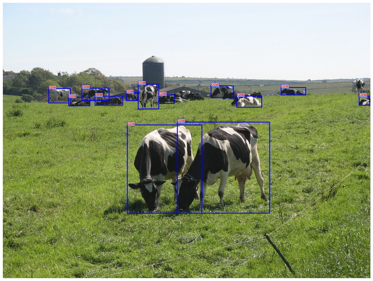
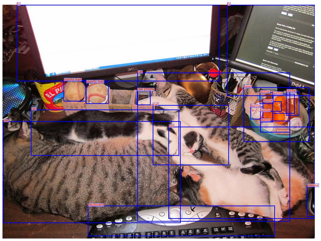
The characteristics of medical datasets likely explain this finding. The objects in natural image datasets, such as MS COCO, show a high variability in scale and quantity due to perspective, camera distance, and the inherent size differences between object classes (Figure 2). Multi-scale fusion benefits such settings by enabling the model to attend to features at different resolutions, capturing objects of varying sizes more effectively. However, in medical datasets like NYU Breast and LUNA16, most images contain a single object and the sizes of these objects are relatively uniform (Figure 6). This contrasts to the MS COCO dataset, showing a broader variation in both the sizes of objects and the number of objects per image. For such medical datasets, the benefits of multi-scale feature fusion are less pronounced. Consequently, in a homogeneous dataset, the additional complexity of multi-scale feature fusion may not translate into better performance.

Notably, in LUNA16, we observed that using the last feature level resulted in a performance drop. This is likely due to the extremely small object size in LUNA16, where all nodules occupy on average 0.6% of the image area (Figure 6 (b)). The last-layer feature map has too low a spatial resolution (i.e. downsized to $16\times 16$ ) to preserve the fine-grained detail necessary for detecting such small objects. This highlights that while multi-scale fusion may not be generally required in medical imaging, selecting an appropriate single feature level, especially one with sufficient spatial resolution, is still critical for detecting very small targets.

Table 3: The performance of Deformable DETRs using different combinations of feature levels. The standard Deformable DETR uses all 4 levels of feature maps from the backbone. Using only the 3rd level feature map for breast NYU and 2nd level feature map for LUNA16, achieves on-par with or even better performance than using multi-level feature fusion.

DatasetFeature Levels $\mathrm{FAUC}^{1}_{10}{\color[rgb]{0,0,0}\definecolor[named]{pgfstrokecolor}{rgb}{0,0,0}\pgfsys@color@gray@stroke{0}\pgfsys@color@gray@fill{0}\pm\mathrm{SD}}$ $\mathrm{AP}_{10}{\color[rgb]{0,0,0}\definecolor[named]{pgfstrokecolor}{rgb}{0,0,0}\pgfsys@color@gray@stroke{0}\pgfsys@color@gray@fill{0}\pm\mathrm{SD}}$ $\mathrm{AP}_{10,50}{\color[rgb]{0,0,0}\definecolor[named]{pgfstrokecolor}{rgb}{0,0,0}\pgfsys@color@gray@stroke{0}\pgfsys@color@gray@fill{0}\pm\mathrm{SD}}$ ${\color[rgb]{0,0,0}\definecolor[named]{pgfstrokecolor}{rgb}{0,0,0}\pgfsys@color@gray@stroke{0}\pgfsys@color@gray@fill{0}L\pm\mathrm{SD}}$ ${\color[rgb]{0,0,0}\definecolor[named]{pgfstrokecolor}{rgb}{0,0,0}\pgfsys@color@gray@stroke{0}\pgfsys@color@gray@fill{0}L_{top10}\pm\mathrm{SD}}$ # paramsGFLOPsNYU $1,2,3,4$ (standard) $0.688\pm 0.012$ $0.677\pm 0.011$ $0.470\pm 0.019$ $0.918\pm 0.005$ $0.855\pm 0.011$ $38.3$ $836$ $1$ $0.637\pm 0.012$ $0.627\pm 0.009$ $0.434\pm 0.009$ $0.924\pm 0.007$ $0.849\pm 0.016$ $35.5$ $734$ $2$ $0.680\pm 0.005$ $0.666\pm 0.009$ $0.467\pm 0.016$ $0.917\pm 0.005$ $0.851\pm 0.012$ $35.6$ $570$ $3$ $0.688\pm 0.004$ $0.675\pm 0.007$ $0.475\pm 0.006$ $0.915\pm 0.010$ $0.858\pm 0.009$ $35.7$ $528$ LUNA $1,2,3,4$ (standard) $0.538\pm 0.013$ $0.390\pm 0.005$ $0.296\pm 0.014$ $0.966\pm 0.002$ $0.680\pm 0.016$ $36.7$ $1225$ $1$ $0.540\pm 0.007$ $0.378\pm 0.022$ $0.267\pm 0.020$ $0.961\pm 0.004$ $0.674\pm 0.022$ $34.2$ $1141$ $2$ $0.548\pm 0.017$ $0.403\pm 0.006$ $0.309\pm 0.008$ $0.965\pm 0.003$ $0.668\pm 0.007$ $34.3$ $1018$ $3$ $0.491\pm 0.015$ $0.290\pm 0.025$ $0.142\pm 0.019$ $0.959\pm 0.005$ $0.637\pm 0.010$ $34.4$ $987$

Number of object queries

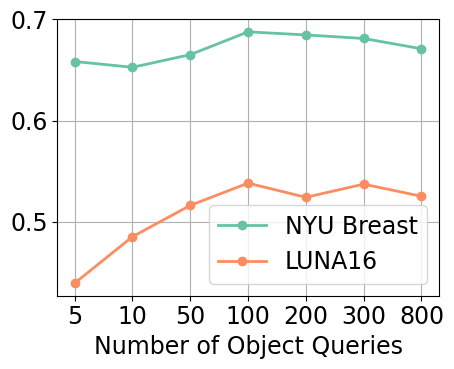
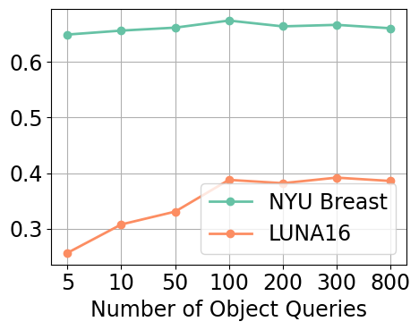
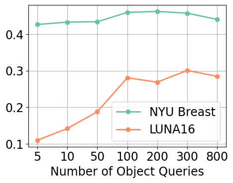
Figure 7(a)-(c) illustrates the impact of increasing the number of object queries from 5 to 800 on detection performance across both the NYU Breast and LUNA16 datasets. Increasing the number of object queries from $5$ to $100$ consistently improves the detection performance. However, further increasing the number of queries beyond 100 results in diminishing returns and even a slight decline in performance. This pattern is consistent on both datasets, although more obvious on LUNA16.

To better understand this behavior, we examined the performance on localization $L$ (cf. Equation 1) and classification $L_{\mathrm{top10}}$ (cf. Equation 2) separately in Figure 7(d). Localization performance ( $L$ ) continues to improve with more object queries, indicating an enhanced ability to correctly localize objects. However, the classification performance ( $L_{\mathrm{top10}}$ ), which measures how many correctly localized boxes rank among the top 10 predictions by classification score, declines beyond 100 queries. This suggests that while more queries increase the likelihood of finding true objects, they also introduce additional false positives that dilute the ranking of true positives.

We hypothesize that having more object queries increases the chances of localizing false positives. More object queries expand the model’s search space, making it more sensitive to subtle features or noise that resemble the characteristics of true objects. This can lead to more false positives being assigned high classification scores, pushing true positives lower in the ranked predictions. This issue is especially relevant in medical imaging, where images typically contain only one or very few objects of interest. In such sparse-object settings, the increased false positive rate from excessive queries can outweigh the benefits of improved localization.

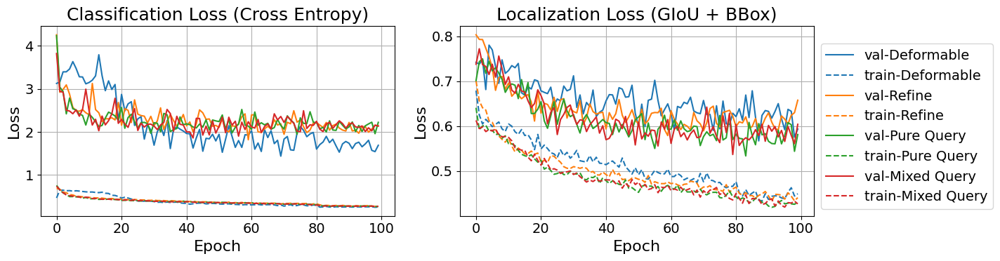
Decoding Techniques

We evaluated two widely used decoding techniques in the DETR family, query initialization and iterative bounding box refinement (IBBR), using a simplified model with design choices achieved through previous results. As shown in Table 4, neither technique significantly improved detection performance across $\mathrm{FAUC}^{1}_{10}$ , $\mathrm{AP}_{10}$ , or $\mathrm{AP}_{10,50}$ for both datasets.

To better understand this outcome, we separately analyzed localization and classification performance using $L$ and $L_{\mathrm{top10}}$ . We found that while these techniques improved localization performance, they adversely affected classification performance. Figure 8 shows training and validation losses for localization (IoU and box regression) and classification (binary cross-entropy). Models equipped with query initialization or IBBR display stronger overfitting, especially in classification loss, compared to the baseline model without these techniques. We hypothesize that this overfitting is due to the limited number of positive objects in our datasets. As the model becomes more effective at localizing regions of interest, it may focus too narrowly on those few positive examples, leading to memorization rather than learning generalizable features. This reduces the model’s ability to accurately distinguish between subtle classes, ultimately weakening the classification performance.

Table 4: Impact of query initialization methods and iterative bounding box refinement (IBBR) on Deformable DETR performance. Detection performance is evaluated on models with the best configuration based on previous experiments for each dataset. Neither query initialization strategies (static, pure, or mixed) nor IBBR consistently improve performance across the three main detection metrics (

\mathrm{FAUC}^{1}_{10}

,

\mathrm{AP}_{10}

,

\mathrm{AP}_{10,50}

). While some configurations improve localization (

L

), classification performance (

L_{\mathrm{top10}}

) generally declines.

DatasetRefinementQuery Initial. $\mathrm{FAUC}^{1}_{10}{\color[rgb]{0,0,0}\definecolor[named]{pgfstrokecolor}{rgb}{0,0,0}\pgfsys@color@gray@stroke{0}\pgfsys@color@gray@fill{0}\pm\mathrm{SD}}$ $\mathrm{AP}_{10}{\color[rgb]{0,0,0}\definecolor[named]{pgfstrokecolor}{rgb}{0,0,0}\pgfsys@color@gray@stroke{0}\pgfsys@color@gray@fill{0}\pm\mathrm{SD}}$ $\mathrm{AP}_{10,50}{\color[rgb]{0,0,0}\definecolor[named]{pgfstrokecolor}{rgb}{0,0,0}\pgfsys@color@gray@stroke{0}\pgfsys@color@gray@fill{0}\pm\mathrm{SD}}$ ${\color[rgb]{0,0,0}\definecolor[named]{pgfstrokecolor}{rgb}{0,0,0}\pgfsys@color@gray@stroke{0}\pgfsys@color@gray@fill{0}L\pm\mathrm{SD}}$ ${\color[rgb]{0,0,0}\definecolor[named]{pgfstrokecolor}{rgb}{0,0,0}\pgfsys@color@gray@stroke{0}\pgfsys@color@gray@fill{0}L_{top10}\pm\mathrm{SD}}$ NYUStatic $0.688\pm 0.004$ $0.675\pm 0.011$ $0.475\pm 0.019$ $0.915\pm 0.010$ $0.858\pm 0.009$ Pure $0.678\pm 0.007$ $0.668\pm 0.011$ $0.474\pm 0.018$ $0.928\pm 0.011$ $0.833\pm 0.015$ Mixed $0.670\pm 0.012$ $0.633\pm 0.010$ $0.443\pm 0.014$ $0.936\pm 0.005$ $0.834\pm 0.012$ $\checkmark$ Static $0.680\pm 0.010$ $0.678\pm 0.012$ $0.470\pm 0.009$ $0.931\pm 0.003$ $0.848\pm 0.009$ $\checkmark$ Pure $0.670\pm 0.010$ $0.670\pm 0.019$ $0.468\pm 0.013$ $0.957\pm 0.008$ $0.838\pm 0.007$ LUNAStatic $0.548\pm 0.017$ $0.403\pm 0.006$ $0.309\pm 0.008$ $0.965\pm 0.003$ $0.668\pm 0.007$ Pure $0.520\pm 0.007$ $0.396\pm 0.006$ $0.298\pm 0.008$ $0.965\pm 0.006$ $0.651\pm 0.008$ Mixed $0.500\pm 0.018$ $0.383\pm 0.007$ $0.291\pm 0.013$ $0.967\pm 0.006$ $0.636\pm 0.022$ $\checkmark$ Static $0.516\pm 0.013$ $0.393\pm 0.017$ $0.303\pm 0.022$ $0.969\pm 0.014$ $0.639\pm 0.004$ $\checkmark$ Pure $0.521\pm 0.015$ $0.399\pm 0.003$ $0.300\pm 0.003$ $0.965\pm 0.007$ $0.635\pm 0.005$

Cases Visualization on NYU Breast

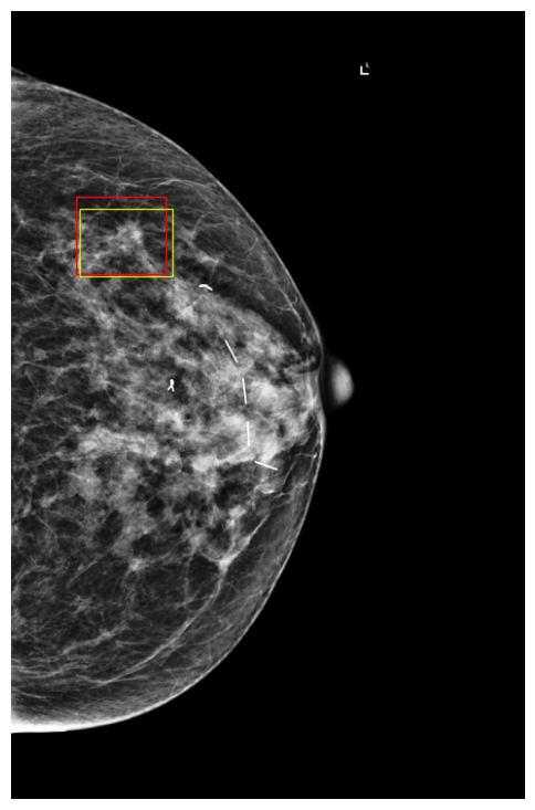
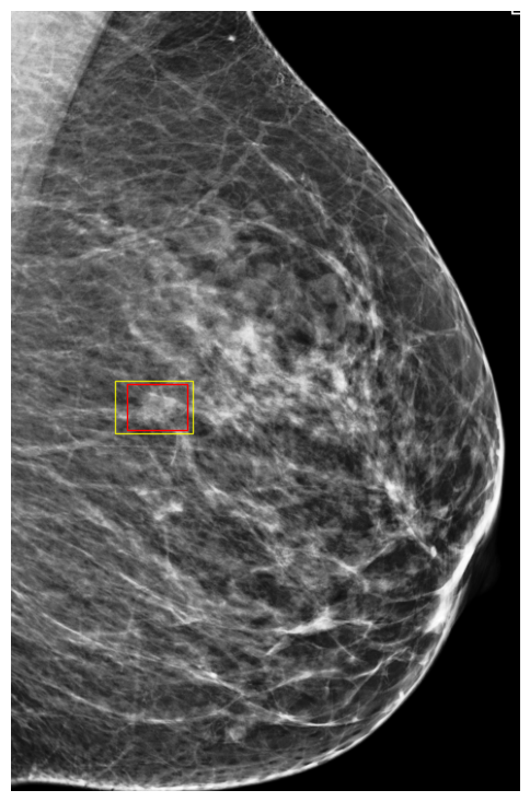
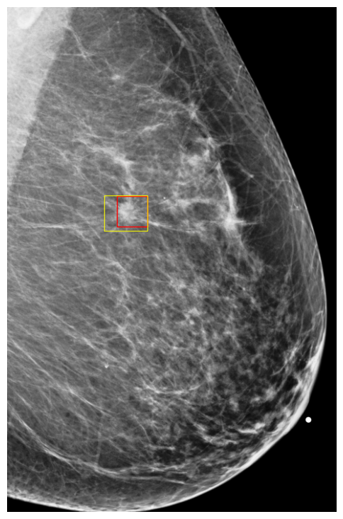
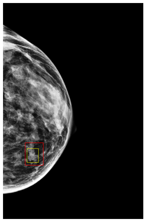
Finally, to better understand how DETR models make predictions, we visualized a few exams along with their classification scores on NYU Breast dataset. Figures 9 and 10 show images in which the model assigned cancerous objects high malignant scores (scores $\geq 0.8$ ) and low scores (scores $\leq 0.1$ ), respectively. We observed that the model correctly localizes abnormal objects in all images. However, it tends to assign high scores to high-density masses featuring non-circumscribed, irregular, or indistinct borders, which are typically indicative of malignancy to the human eye. In contrast, the model usually assigns low scores to low-density masses with circumscribed borders, which can easily be confused with benign cases (Lee et al., 2018).

5 Conclusions

In this study, we investigated the impact of common design choices in Deformable DETR (Zhu et al., 2020) on object detection performance in medical imaging, using two representative datasets: the NYU Breast Cancer Screening Dataset and LUNA16. We found that all the design choices we experimented with need to be reconsidered, and simpler architectures typically lead to better performance on medical dataset.

Additionally, our findings suggest that the model tends to struggle more with correctly classifying detected objects than with localizing them. Many design choices developed for natural image detection, such as query initialization, multi-scale feature fusion, and bounding box refinement, are primarily aimed at improving localization. However, since classification appears to be the more challenging component in medical imaging, these localization-focused techniques may offer limited benefit and, in some cases, even hinder performance.

Future research should focus on developing architectures specifically tailored to the characteristics of medical imaging. This includes improving the model’s ability to extract subtle visual cues that are often critical for classification, such as texture variations, tissue density changes, irregular borders, and microcalcifications. Another important direction is designing architectures that can efficiently process full-resolution images, allowing the model to leverage detailed information in relevant regions while minimizing the influence of background areas. Moreover, addressing overfitting in classification tasks, particularly in datasets with limited positive samples, requires the integration of effective regularization techniques to improve generalization and robustness.

6 Limitations and future work

Our study has several limitations. First, while our results demonstrate that simplified DETR configurations perform well on medical imaging tasks, future studies should explore additional architectural designs within the DETR family to validate and extend these findings, for example, constrastive denoising training in DINO (Zhang et al., 2022) and anchors in Anchor-DETR (Wang et al., 2022). Second, our experiments were conducted primarily on the NYU Breast Cancer Screening Dataset and LUNA16 for lung nodule detection. While these datasets capture important aspects of medical imaging, future studies should evaluate model performance across a broader set of imaging modalities and clinical tasks, such as brain MRI, ultrasound, or multi-phase CT, to assess the generalizability of our conclusions.

Acknowledgments

This work was supported in part by grants from the National Institutes of Health (P41EB017183), the National Science Foundation (1922658), the Gordon and Betty Moore Foundation (9683), and the Mary Kay Ash Foundation (05-22). We also appreciate the support of Nvidia Corporation with the donation of some of the GPUs used in this research.

Ethical Standards

This retrospective study was approved by the NYU Langone Health Institutional Review Board (ID#i18-00712_CR3) and is compliant with the Health Insurance Portability and Accountability Act. Informed consent was waived since the study presents no more than minimal risk.

Conflicts of Interest

The authors do not declare any conflicts of interest.

Data availability

Our internal (NYU Langone Health) dataset is not publicly available due to internal data transfer policies. We released a data report on data curation and preprocessing to encourage reproducibility. The data report can be accessed at this link.

References

Bandos et al. (2009) Andriy I Bandos, Howard E Rockette, Tao Song, and David Gur. Area under the free-response ROC curve (FROC) and a related summary index. Biometrics, 65(1):247–256, 2009.
Carion et al. (2020) Nicolas Carion, Francisco Massa, Gabriel Synnaeve, Nicolas Usunier, Alexander Kirillov, and Sergey Zagoruyko. End-to-end object detection with transformers. In Computer Vision–ECCV 2020: 16th European Conference, Glasgow, UK, August 23–28, 2020, Proceedings, Part I 16, pages 213–229. Springer, 2020.
Chen et al. (2021) Jieneng Chen, Yongyi Lu, Qihang Yu, Xiangde Luo, Ehsan Adeli, Yan Wang, Le Lu, Alan L Yuille, and Yuyin Zhou. Transunet: Transformers make strong encoders for medical image segmentation. arXiv preprint arXiv:2102.04306, 2021.
Chen et al. (2022a) Qiang Chen, Xiaokang Chen, Gang Zeng, and Jingdong Wang. Group DETR: Fast training convergence with decoupled one-to-many label assignment. arXiv preprint arXiv:2207.13085, 2022a.
Chen et al. (2022b) Xiaokang Chen, Fangyun Wei, Gang Zeng, and Jingdong Wang. Conditional DETRv2: Efficient detection transformer with box queries. arXiv preprint arXiv:2207.08914, 2022b.
Dai et al. (2021a) Xiyang Dai, Yinpeng Chen, Jianwei Yang, Pengchuan Zhang, Lu Yuan, and Lei Zhang. Dynamic DETR: End-to-end object detection with dynamic attention. In Proceedings of the IEEE/CVF International Conference on Computer Vision, pages 2988–2997, 2021a.
Dai et al. (2021b) Yin Dai, Yifan Gao, and Fayu Liu. Transmed: Transformers advance multi-modal medical image classification. Diagnostics, 11(8):1384, 2021b.
Dosovitskiy et al. (2020) Alexey Dosovitskiy, Lucas Beyer, Alexander Kolesnikov, Dirk Weissenborn, Xiaohua Zhai, Thomas Unterthiner, Mostafa Dehghani, Matthias Minderer, Georg Heigold, Sylvain Gelly, et al. An image is worth 16x16 words: Transformers for image recognition at scale. arXiv preprint arXiv:2010.11929, 2020.
Everingham et al. (2010) Mark Everingham, Luc Van Gool, Christopher KI Williams, John Winn, and Andrew Zisserman. The pascal visual object classes (VOC) challenge. International Journal of Computer Vision, 88:303–338, 2010.
Galdran et al. (2021) Adrian Galdran, Gustavo Carneiro, and Miguel A González Ballester. Balanced-mixup for highly imbalanced medical image classification. In Medical Image Computing and Computer Assisted Intervention–MICCAI 2021: 24th International Conference, Strasbourg, France, September 27–October 1, 2021, Proceedings, Part V 24, pages 323–333. Springer, 2021.
Garrucho et al. (2023) Lidia Garrucho, Kaisar Kushibar, Richard Osuala, Oliver Diaz, Alessandro Catanese, Javier del Riego, Maciej Bobowicz, Fredrik Strand, Laura Igual, and Karim Lekadir. High-resolution synthesis of high-density breast mammograms: Application to improved fairness in deep learning based mass detection. Frontiers in Oncology, 12:1044496, 01 2023. .
Geman et al. (1992) Stuart Geman, Elie Bienenstock, and René Doursat. Neural networks and the bias/variance dilemma. Neural Computation, 4(1):1–58, 1992.
Girshick et al. (2014) Ross Girshick, Jeff Donahue, Trevor Darrell, and Jitendra Malik. Rich feature hierarchies for accurate object detection and semantic segmentation. In Proceedings of the IEEE Conference on Computer Vision and Pattern Recognition, pages 580–587, 2014.
He et al. (2017) Kaiming He, Georgia Gkioxari, Piotr Dollár, and Ross Girshick. Mask r-cnn. In Proceedings of the IEEE International Conference on Computer Vision, pages 2961–2969, 2017.
Heath et al. (2001) Michael Heath, Kevin Bowyer, Daniel Kopans, Richard Moore, and W. Philip Kegelmeyer. The digital database for screening mammography. In M.J. Yaffe, editor, Proceedings of the Fifth International Workshop on Digital Mammography, pages 212–218. Medical Physics Publishing, 2001. ISBN 1-930524-00-5.
Jailin et al. (2023) Clément Jailin, Răzvan Iordache, Pablo Milioni de Carvalho, Salwa Ahmed, Engy Sattar, Amr Moustafa, Mohammed Gomaa, Rashaa Kamal, and Laurence Vancamberg. AI-based cancer detection model for contrast-enhanced mammography. Bioengineering, 10:974, 08 2023. .
Johnson et al. (2019) Alistair EW Johnson, Tom J Pollard, Nathaniel R Greenbaum, Matthew P Lungren, Chih-ying Deng, Yifan Peng, Zhiyong Lu, Roger G Mark, Seth J Berkowitz, and Steven Horng. Mimic-cxr-jpg, a large publicly available database of labeled chest radiographs. arXiv preprint arXiv:1901.07042, 2019.
Kolchev et al. (2022) Alexey Kolchev, D. Pasynkov, Ivan Egoshin, Ivan Kliouchkin, Olga Pasynkova, and Dmitrii Tumakov. YOLOv4-based CNN model versus nested contours algorithm in the suspicious lesion detection on the mammography image: A direct comparison in the real clinical settings. Journal of Imaging, 8:88, 03 2022. .
Konz et al. (2023) Nicholas Konz, Mateusz Buda, Hanxue Gu, Ashirbani Saha, Jichen Yang, Jakub Chledowski, Jungkyu Park, Jan Witowski, Krzysztof J. Geras, Yoel Shoshan, Flora Gilboa-Solomon, Daniel Khapun, Vadim Ratner, Ella Barkan, Michal Ozery-Flato, Robert Martí, Akinyinka Omigbodun, Chrysostomos Marasinou, Noor Nakhaei, William Hsu, Pranjal Sahu, Md Belayat Hossain, Juhun Lee, Carlos Santos, Artur Przelaskowski, Jayashree Kalpathy-Cramer, Benjamin Bearce, Kenny Cha, Keyvan Farahani, Nicholas Petrick, Lubomir Hadjiiski, Karen Drukker, III Armato, Samuel G., and Maciej A. Mazurowski. A Competition, Benchmark, Code, and Data for Using Artificial Intelligence to Detect Lesions in Digital Breast Tomosynthesis. JAMA Network Open, 6(2):e230524–e230524, 02 2023. ISSN 2574-3805. . URL https://doi.org/10.1001/jamanetworkopen.2023.0524.
Kuhn (1955) Harold W Kuhn. The hungarian method for the assignment problem. Naval Research Logistics Quarterly, 2(1-2):83–97, 1955.
Lee et al. (2018) Christoph I. Lee, Constance D. Lehman, Lawrence W. Bassett, and Lonie R. Salkowski. 204Mass with Indistinct Margins. In Breast Imaging. Oxford University Press, 01 2018. ISBN 9780190270261. . URL https://doi.org/10.1093/med/9780190270261.003.0024.
Li et al. (2023) Manyu Li, Shichang Liu, Zihan Wang, Xin Li, Zezhong Yan, Renping Zhu, and Zhijiang Wan. MyopiaDETR: End-to-end pathological myopia detection based on transformer using 2D fundus images. Frontiers in Neuroscience, 17:1130609, 2023.
Lin et al. (2022) Junyu Lin, Xiaofeng Mao, Yuefeng Chen, Lei Xu, Yuan He, and Hui Xue. D^ 2ETR: Decoder-only DETR with computationally efficient cross-scale attention. arXiv preprint arXiv:2203.00860, 2022.
Lin et al. (2014) Tsung-Yi Lin, Michael Maire, Serge Belongie, James Hays, Pietro Perona, Deva Ramanan, Piotr Dollár, and C Lawrence Zitnick. Microsoft COCO: Common objects in context. In Computer Vision–ECCV 2014: 13th European Conference, Zurich, Switzerland, September 6-12, 2014, Proceedings, Part V 13, pages 740–755. Springer, 2014.
Lin et al. (2017) Tsung-Yi Lin, Priya Goyal, Ross Girshick, Kaiming He, and Piotr Dollár. Focal loss for dense object detection. In Proceedings of the IEEE International Conference on Computer Vision, pages 2980–2988, 2017.
Liu et al. (2022) Shilong Liu, Feng Li, Hao Zhang, Xiao Yang, Xianbiao Qi, Hang Su, Jun Zhu, and Lei Zhang. Dab-DETR: Dynamic anchor boxes are better queries for DETR. arXiv preprint arXiv:2201.12329, 2022.
Liu et al. (2021) Ze Liu, Yutong Lin, Yue Cao, Han Hu, Yixuan Wei, Zheng Zhang, Stephen Lin, and Baining Guo. Swin transformer: Hierarchical vision transformer using shifted windows. In Proceedings of the IEEE/CVF International Conference on Computer Vision, pages 10012–10022, 2021.
Loshchilov and Hutter (2017) Ilya Loshchilov and Frank Hutter. Decoupled weight decay regularization. arXiv preprint arXiv:1711.05101, 2017.
Mathai et al. (2022) Tejas Sudharshan Mathai, Sungwon Lee, Daniel C Elton, Thomas C Shen, Yifan Peng, Zhiyong Lu, and Ronald M Summers. Lymph node detection in t2 mri with transformers. In Medical Imaging 2022: Computer-Aided Diagnosis, volume 12033, pages 855–859. SPIE, 2022.
Moawad et al. (2023) Ahmed W Moawad, Anastasia Janas, Ujjwal Baid, Divya Ramakrishnan, Leon Jekel, Kiril Krantchev, Harrison Moy, Rachit Saluja, Klara Osenberg, Klara Wilms, et al. The brain tumor segmentation (brats-mets) challenge 2023: Brain metastasis segmentation on pre-treatment mri. arXiv preprint arXiv:2306.00838, 2023.
Petrick et al. (2013) Nicholas Petrick, Berkman Sahiner, Samuel G Armato III, Alberto Bert, Loredana Correale, Silvia Delsanto, Matthew T Freedman, David Fryd, David Gur, Lubomir Hadjiiski, et al. Evaluation of computer-aided detection and diagnosis systems a. Medical Physics, 40(8):087001, 2013.
Prangemeier et al. (2020) Tim Prangemeier, Christoph Reich, and Heinz Koeppl. Attention-based transformers for instance segmentation of cells in microstructures. In 2020 IEEE International Conference on Bioinformatics and Biomedicine (BIBM), pages 700–707. IEEE, 2020.
Redmon et al. (2016) Joseph Redmon, Santosh Divvala, Ross Girshick, and Ali Farhadi. You only look once: Unified, real-time object detection. In Proceedings of the IEEE Conference on Computer Vision and Pattern Recognition, pages 779–788, 2016.
Rezatofighi et al. (2019) Hamid Rezatofighi, Nathan Tsoi, JunYoung Gwak, Amir Sadeghian, Ian Reid, and Silvio Savarese. Generalized intersection over union. June 2019.
Richter et al. (2021) Mats L. Richter, Wolf Byttner, Ulf Krumnack, Anna Wiedenroth, Ludwig Schallner, and Justin Shenk. (Input) Size Matters for CNN Classifiers, page 133–144. Springer International Publishing, 2021. ISBN 9783030863401. . URL http://dx.doi.org/10.1007/978-3-030-86340-1_11.
Roh et al. (2021) Byungseok Roh, JaeWoong Shin, Wuhyun Shin, and Saehoon Kim. Sparse DETR: Efficient end-to-end object detection with learnable sparsity. arXiv preprint arXiv:2111.14330, 2021.
Sabottke and Spieler (2020) Carl F Sabottke and Bradley M Spieler. The effect of image resolution on deep learning in radiography. Radiology: Artificial Intelligence, 2(1):e190015, 2020.
Salton (1983) Gerard Salton. Introduction to modern information retrieval. McGraw-Hill, 1983.
Setio et al. (2017) Arnaud Arindra Adiyoso Setio, Alberto Traverso, Thomas De Bel, Moira SN Berens, Cas Van Den Bogaard, Piergiorgio Cerello, Hao Chen, Qi Dou, Maria Evelina Fantacci, Bram Geurts, et al. Validation, comparison, and combination of algorithms for automatic detection of pulmonary nodules in computed tomography images: the luna16 challenge. Medical image analysis, 42:1–13, 2017.
Shen et al. (2021) Zhiqiang Shen, Rongda Fu, Chaonan Lin, and Shaohua Zheng. COTR: Convolution in transformer network for end to end polyp detection. In 2021 7th International Conference on Computer and Communications (ICCC), pages 1757–1761. IEEE, 2021.
Thambawita et al. (2021) Vajira Thambawita, Inga Strümke, Steven A Hicks, Pål Halvorsen, Sravanthi Parasa, and Michael A Riegler. Impact of image resolution on deep learning performance in endoscopy image classification: an experimental study using a large dataset of endoscopic images. Diagnostics, 11(12):2183, 2021.
Touvron et al. (2021) Hugo Touvron, Matthieu Cord, Matthijs Douze, Francisco Massa, Alexandre Sablayrolles, and Hervé Jégou. Training data-efficient image transformers & distillation through attention. In International Conference on Machine Learning, pages 10347–10357. PMLR, 2021.
Valanarasu et al. (2021) Jeya Maria Jose Valanarasu, Poojan Oza, Ilker Hacihaliloglu, and Vishal M Patel. Medical transformer: Gated axial-attention for medical image segmentation. In Medical Image Computing and Computer Assisted Intervention–MICCAI 2021: 24th International Conference, Strasbourg, France, September 27–October 1, 2021, Proceedings, Part I 24, pages 36–46. Springer, 2021.
Vaswani et al. (2017) Ashish Vaswani, Noam Shazeer, Niki Parmar, Jakob Uszkoreit, Llion Jones, Aidan N Gomez, Łukasz Kaiser, and Illia Polosukhin. Attention is all you need. Advances in Neural Information Processing Systems, 30, 2017.
Wang et al. (2018) Pu Wang, Xiao Xiao, Jeremy R Glissen Brown, Tyler M Berzin, Mengtian Tu, Fei Xiong, Xiao Hu, Peixi Liu, Yan Song, Di Zhang, et al. Development and validation of a deep-learning algorithm for the detection of polyps during colonoscopy. Nature Biomedical Engineering, 2(10):741–748, 2018.
Wang et al. (2017) Xiaosong Wang, Yifan Peng, Le Lu, Zhiyong Lu, Mohammadhadi Bagheri, and Ronald M Summers. Chestx-ray8: Hospital-scale chest x-ray database and benchmarks on weakly-supervised classification and localization of common thorax diseases. In Proceedings of the IEEE Conference on Computer Vision and Pattern Recognition, pages 2097–2106, 2017.
Wang et al. (2022) Yingming Wang, Xiangyu Zhang, Tong Yang, and Jian Sun. Anchor DETR: Query design for transformer-based detector. In Proceedings of the AAAI Conference on Artificial Intelligence, volume 36, pages 2567–2575, 2022.
Wu et al. (2019) Nan Wu, Jason Phang, Jungkyu Park, Yiqiu Shen, S.G. Kim, Laura Heacock, Linda Moy, Kyunghyun Cho, and Krzyszrof J. Geras. The NYU breast cancer screening dataset v1.0. Tech. rep., New York Univ., New York, NY, USA, 2019.
Yao et al. (2021) Zhuyu Yao, Jiangbo Ai, Boxun Li, and Chi Zhang. Efficient DETR: improving end-to-end object detector with dense prior. arXiv preprint arXiv:2104.01318, 2021.
Yu et al. (2022) Xiang Yu, Qinghua Zhou, Shuihua Wang, and Yu-Dong Zhang. A systematic survey of deep learning in breast cancer. International Journal of Intelligent Systems, 37(1):152–216, 2022.
Zeng et al. (2022) Nianyin Zeng, Peishu Wu, Zidong Wang, Han Li, Weibo Liu, and Xiaohui Liu. A small-sized object detection oriented multi-scale feature fusion approach with application to defect detection. IEEE Transactions on Instrumentation and Measurement, 71:1–14, 2022.
Zhang et al. (2022) Hao Zhang, Feng Li, Shilong Liu, Lei Zhang, Hang Su, Jun Zhu, Lionel M Ni, and Heung-Yeung Shum. Dino: DETR with improved denoising anchor boxes for end-to-end object detection. arXiv preprint arXiv:2203.03605, 2022.
Zheng et al. (2022) Yi Zheng, Rushin H Gindra, Emily J Green, Eric J Burks, Margrit Betke, Jennifer E Beane, and Vijaya B Kolachalama. A graph-transformer for whole slide image classification. IEEE Transactions on Medical Imaging, 41(11):3003–3015, 2022.
Zhou et al. (2021) Wujie Zhou, Xinyang Lin, Jingsheng Lei, Lu Yu, and Jenq-Neng Hwang. MFFENet: Multiscale feature fusion and enhancement network for rgb–thermal urban road scene parsing. IEEE Transactions on Multimedia, 24:2526–2538, 2021.
Zhu et al. (2020) Xizhou Zhu, Weijie Su, Lewei Lu, Bin Li, Xiaogang Wang, and Jifeng Dai. Deformable DETR: Deformable transformers for end-to-end object detection. arXiv preprint arXiv:2010.04159, 2020.
Zong et al. (2023) Zhuofan Zong, Guanglu Song, and Yu Liu. DETRs with collaborative hybrid assignments training. In Proceedings of the IEEE/CVF International Conference on Computer Vision, pages 6748–6758, 2023.

A DETR architecture

A.1 Multi-head self-attention (MHSA)

A standard MHSA with $M$ heads is defined as:

		$\displaystyle\mathrm{MHSA}(Q,K,V)$		(3)
		$\displaystyle=\sum_{m=1}^{M}W_{mo}\left[\mathrm{softmax}\left(\frac{QW_{mq}(KW_{mk})^{T}}{\sqrt{d/M}}\right)VW_{mv}\right].$		(4)

The $K$ , $Q$ and $V$ represent the query, key, and value matrices respectively, defined with respect to input feature map $x_{f}\in\mathbb{R}^{WH\times d}$ and its positional embedding $x_{p}\in\mathbb{R}^{WH\times d}$ :

Q=x_{f}+x_{p},K=x_{f}+x_{p},V=x_{f}.

(5)

$W_{mq},W_{mk},W_{mv}\in\mathbb{R}^{d\times d/M}$ linearly transforms $K,Q,V$ in the $m$ -th head and $W_{mo}\in\mathbb{R}^{d/M\times d}$ .

A.2 Multi-head (MH) cross-attention

The MH cross-attention module performs the same computation as the MHSA defined in 3, except that $K,Q,V$ are defined based on two different sets of tokens. The queries $Q$ are defined by the object queries $q=q_{c}+q_{p}$ , where $q_{p}$ and $q_{c}$ are the positional embedding and the content embedding of the object queries. The keys $K$ are defined by the encoder features $x_{enc}+x_{p}$ . Specifically,

Q=q_{c}+q_{p},K=x_{enc}+x_{p},V=q_{c}.

(6)

A.3 Set prediction loss

DETR uses a set prediction loss that enables end-to-end training without non-maximum suppression (NMS). DETR produces a fixed number of predictions per image $N$ , and $N$ is set to be significantly larger than the maximum possible number of objects in the image. Let $\{\hat{y}_{i}=(\hat{c}_{i},\hat{b}_{i})\}_{N}$ be all pairs of class and box predictions. The set of $N$ labels is $\{y_{i}=(c_{i},b_{i})\}_{N}$ where each ground truth label represents an object in the image. If there are fewer objects than $N$ , the rest of the labels are empty classes $(0,\emptyset)$ . The set prediction loss is computed in two steps. The first step is to find a permutation $\sigma$ on the set of labels $\{y_{i}\}$ that minimizes the matching loss, defined as below:

\mathbf{\hat{\sigma}}=\arg\min_{\sigma\in\Sigma_{N}}\sum_{N}^{i}\mathcal{L}_{match}(\hat{y}_{i},y_{\sigma(i)}).

The matching loss for a matching pair is a linear combination of classification loss, box regression loss and GIoU loss (Rezatofighi et al., 2019). The classification loss is a standard focal loss (Lin et al., 2017). The regression loss and the GIoU loss are only applied to non-empty labels. It is defined as the following:

\mathcal{L}_{match}(\hat{y}_{i},y_{\sigma(i)})=W_{cls}\mathcal{L}_{cls}(\hat{c}_{i},c_{\sigma(i)})

+1_{b\neq\emptyset}\left(W_{l1}\mathcal{L}_{l1}(\hat{b}_{i},b_{\sigma(i)})+W_{giou}\mathcal{L}_{giou}(\hat{b}_{i},b_{\sigma(i)})\right),

where $W_{cls},W_{l1},W_{giou}$ are scalar coefficients that are tuned as hyperparameters to balance the scale of different losses. The Hungarian algorithm (Kuhn, 1955) can efficiently find the optimal match $\hat{\sigma}$ . The second step is to minimize the loss function $\sum_{N}^{i}\mathcal{L}_{match}(\hat{y}_{i},y_{\hat{\sigma}(i)})$ with the permutation $\hat{\sigma}$ on the label set.

DETR also utilizes auxiliary loss in each decoder layer to provide stronger supervision. At the end of each decoder layer, it predicts $N$ boxes and class scores with MLP prediction heads. All prediction heads share weights. The above two steps, the matching step and the Hungarian loss minimization, are applied to each decoder layer’s output. In inference, only the output of the last layer is used as the final prediction.

B Deformable DETR architecture

B.1 Deformable multi-head self-attention

Formally, deformable MHSA for a single query $q\in\mathbb{R}^{d}$ in the feature map is given by:

	$\displaystyle\mathrm{Deform\_MHSA}(Q_{q},K,V)$		(7)
	$\displaystyle=\sum_{m=1}^{M}W_{mo}\left[\mathrm{softmax}\left(K_{q}W_{mk}\right)V_{q}W_{mv}\right]$		(8)

The $Q$ , $K$ and $V$ represent the query, key, and value matrices respectively, defined as the following,

	$\displaystyle Q=x_{f}+x_{p},$		(9)
	$\displaystyle Q_{q}=q,$		(10)
	$\displaystyle K_{q}=\delta(K,q)\in\mathbb{R}^{k\times d},$		(11)
	$\displaystyle V_{q}=\delta(V,q)\in\mathbb{R}^{k\times d}.$		(12)

The key sampling function $\delta$ samples the $k$ keys from the full set of keys $K=x_{f}+x_{p}$ by generating the sampling offsets $\Delta p$ with respect to reference points $p_{q}$ : $\delta(K,q)=K(p_{q}+\Delta p)$ . The sampling offsets are obtained by linear transformation of the query $q$ .

C Iterative Bounding Box Refinement Technique

In the standard Deformable DETR, a 2D reference point $r_{q}\in[0,1]^{2}$ for each object query $q$ is derived from its learnable positional embedding $p_{q}$ via a linear layer

r_{q}=\mathrm{linear}(p_{q}).

Throughout the decoder, the locations of these reference points remain constant. They are updated based on the learnable positional embedding $p_{q}$ when a backward pass is completed. Formally, let $r_{q}^{i}$ be the reference points of an object query $q$ in the i-th decoder layer. In standard Deformable DETR,

r_{q}^{1}=r_{q}^{2}=\ldots=r_{q}^{6}.

In IBBR, the reference points $r_{q}^{i}$ in i-th decoder layer are refined based on the previous reference points $r_{q}^{i-1}$ and the offsets predicted by the auxiliary prediction head, which is a Multi-layer Perceptron (MLP). MLP is defined by three fully connected layers, which transform the output embeddings of the transformer into the desired bounding box coordinates.

r_{q}^{i}=S(\mathrm{linear}^{-1}(S^{-1}(r_{q}^{i-1}))+\mathrm{MLP}(x_{dec}^{i})),

where $S$ and $S^{-1}$ represent the sigmoid function and its inverse, and $x^{i}_{dec}$ is the output of the i-th decoder layer.

D Backbone Pre-training

We pretrained the Swin-T Transfromer backbone with a cancer classification task on our dataset. This classification task is a binary multi-label classification that predicts two scores indicating if an input image contains benign lesions and/or malignant lesions.

E Hyperparameter Tuning

Our method for hyper-parameter tuning is random search. We tuned the following hyperparameters and their ranges on quarter-resolution images:

•
learning rate $\eta\in 10^{[3,5.5]}$ ,
•
scale of the backbone learning rate $s\in[1,0.01]$ (backbone learning rate = $s\times\eta$ ),
•
weight decay $\lambda\in 10^{[3,6]}$ ,
•
number of object queries $N\in[10,200]$ ,
•
two hyperparameters $\alpha$ and $\gamma$ in the focal loss $\alpha\in[0,1]$ , $\gamma\in[0,3]$ ,
•
the coefficients on classification loss and GIoU loss $\in[0,1]$ .

We train $80$ jobs in total and choose the best model based on $\mathrm{FAUC}^{1}_{10}$ .

[bib.bib1] Bandos et al. (2009) Andriy I Bandos, Howard E Rockette, Tao Song, and David Gur. Area under the free-response ROC curve (FROC) and a related summary index. Biometrics, 65(1):247–256, 2009.

[bib.bib2] Carion et al. (2020) Nicolas Carion, Francisco Massa, Gabriel Synnaeve, Nicolas Usunier, Alexander Kirillov, and Sergey Zagoruyko. End-to-end object detection with transformers. In Computer Vision–ECCV 2020: 16th European Conference, Glasgow, UK, August 23–28, 2020, Proceedings, Part I 16, pages 213–229. Springer, 2020.

[bib.bib3] Chen et al. (2021) Jieneng Chen, Yongyi Lu, Qihang Yu, Xiangde Luo, Ehsan Adeli, Yan Wang, Le Lu, Alan L Yuille, and Yuyin Zhou. Transunet: Transformers make strong encoders for medical image segmentation. arXiv preprint arXiv:2102.04306, 2021.

[bib.bib4] Chen et al. (2022a) Qiang Chen, Xiaokang Chen, Gang Zeng, and Jingdong Wang. Group DETR: Fast training convergence with decoupled one-to-many label assignment. arXiv preprint arXiv:2207.13085, 2022a.

[bib.bib5] Chen et al. (2022b) Xiaokang Chen, Fangyun Wei, Gang Zeng, and Jingdong Wang. Conditional DETRv2: Efficient detection transformer with box queries. arXiv preprint arXiv:2207.08914, 2022b.

[bib.bib6] Dai et al. (2021a) Xiyang Dai, Yinpeng Chen, Jianwei Yang, Pengchuan Zhang, Lu Yuan, and Lei Zhang. Dynamic DETR: End-to-end object detection with dynamic attention. In Proceedings of the IEEE/CVF International Conference on Computer Vision, pages 2988–2997, 2021a.

[bib.bib7] Dai et al. (2021b) Yin Dai, Yifan Gao, and Fayu Liu. Transmed: Transformers advance multi-modal medical image classification. Diagnostics, 11(8):1384, 2021b.

[bib.bib8] Dosovitskiy et al. (2020) Alexey Dosovitskiy, Lucas Beyer, Alexander Kolesnikov, Dirk Weissenborn, Xiaohua Zhai, Thomas Unterthiner, Mostafa Dehghani, Matthias Minderer, Georg Heigold, Sylvain Gelly, et al. An image is worth 16x16 words: Transformers for image recognition at scale. arXiv preprint arXiv:2010.11929, 2020.

[bib.bib9] Everingham et al. (2010) Mark Everingham, Luc Van Gool, Christopher KI Williams, John Winn, and Andrew Zisserman. The pascal visual object classes (VOC) challenge. International Journal of Computer Vision, 88:303–338, 2010.

[bib.bib10] Galdran et al. (2021) Adrian Galdran, Gustavo Carneiro, and Miguel A González Ballester. Balanced-mixup for highly imbalanced medical image classification. In Medical Image Computing and Computer Assisted Intervention–MICCAI 2021: 24th International Conference, Strasbourg, France, September 27–October 1, 2021, Proceedings, Part V 24, pages 323–333. Springer, 2021.

[bib.bib11] Garrucho et al. (2023) Lidia Garrucho, Kaisar Kushibar, Richard Osuala, Oliver Diaz, Alessandro Catanese, Javier del Riego, Maciej Bobowicz, Fredrik Strand, Laura Igual, and Karim Lekadir. High-resolution synthesis of high-density breast mammograms: Application to improved fairness in deep learning based mass detection. Frontiers in Oncology, 12:1044496, 01 2023. .

[bib.bib12] Geman et al. (1992) Stuart Geman, Elie Bienenstock, and René Doursat. Neural networks and the bias/variance dilemma. Neural Computation, 4(1):1–58, 1992.

[bib.bib13] Girshick et al. (2014) Ross Girshick, Jeff Donahue, Trevor Darrell, and Jitendra Malik. Rich feature hierarchies for accurate object detection and semantic segmentation. In Proceedings of the IEEE Conference on Computer Vision and Pattern Recognition, pages 580–587, 2014.

[bib.bib14] He et al. (2017) Kaiming He, Georgia Gkioxari, Piotr Dollár, and Ross Girshick. Mask r-cnn. In Proceedings of the IEEE International Conference on Computer Vision, pages 2961–2969, 2017.

[bib.bib15] Heath et al. (2001) Michael Heath, Kevin Bowyer, Daniel Kopans, Richard Moore, and W. Philip Kegelmeyer. The digital database for screening mammography. In M.J. Yaffe, editor, Proceedings of the Fifth International Workshop on Digital Mammography, pages 212–218. Medical Physics Publishing, 2001. ISBN 1-930524-00-5.

[bib.bib16] Jailin et al. (2023) Clément Jailin, Răzvan Iordache, Pablo Milioni de Carvalho, Salwa Ahmed, Engy Sattar, Amr Moustafa, Mohammed Gomaa, Rashaa Kamal, and Laurence Vancamberg. AI-based cancer detection model for contrast-enhanced mammography. Bioengineering, 10:974, 08 2023. .

[bib.bib17] Johnson et al. (2019) Alistair EW Johnson, Tom J Pollard, Nathaniel R Greenbaum, Matthew P Lungren, Chih-ying Deng, Yifan Peng, Zhiyong Lu, Roger G Mark, Seth J Berkowitz, and Steven Horng. Mimic-cxr-jpg, a large publicly available database of labeled chest radiographs. arXiv preprint arXiv:1901.07042, 2019.

[bib.bib18] Kolchev et al. (2022) Alexey Kolchev, D. Pasynkov, Ivan Egoshin, Ivan Kliouchkin, Olga Pasynkova, and Dmitrii Tumakov. YOLOv4-based CNN model versus nested contours algorithm in the suspicious lesion detection on the mammography image: A direct comparison in the real clinical settings. Journal of Imaging, 8:88, 03 2022. .

[bib.bib19] Konz et al. (2023) Nicholas Konz, Mateusz Buda, Hanxue Gu, Ashirbani Saha, Jichen Yang, Jakub Chledowski, Jungkyu Park, Jan Witowski, Krzysztof J. Geras, Yoel Shoshan, Flora Gilboa-Solomon, Daniel Khapun, Vadim Ratner, Ella Barkan, Michal Ozery-Flato, Robert Martí, Akinyinka Omigbodun, Chrysostomos Marasinou, Noor Nakhaei, William Hsu, Pranjal Sahu, Md Belayat Hossain, Juhun Lee, Carlos Santos, Artur Przelaskowski, Jayashree Kalpathy-Cramer, Benjamin Bearce, Kenny Cha, Keyvan Farahani, Nicholas Petrick, Lubomir Hadjiiski, Karen Drukker, III Armato, Samuel G., and Maciej A. Mazurowski. A Competition, Benchmark, Code, and Data for Using Artificial Intelligence to Detect Lesions in Digital Breast Tomosynthesis. JAMA Network Open, 6(2):e230524–e230524, 02 2023. ISSN 2574-3805. . URL https://doi.org/10.1001/jamanetworkopen.2023.0524.

[bib.bib20] Kuhn (1955) Harold W Kuhn. The hungarian method for the assignment problem. Naval Research Logistics Quarterly, 2(1-2):83–97, 1955.

[bib.bib21] Lee et al. (2018) Christoph I. Lee, Constance D. Lehman, Lawrence W. Bassett, and Lonie R. Salkowski. 204Mass with Indistinct Margins. In Breast Imaging. Oxford University Press, 01 2018. ISBN 9780190270261. . URL https://doi.org/10.1093/med/9780190270261.003.0024.

[bib.bib22] Li et al. (2023) Manyu Li, Shichang Liu, Zihan Wang, Xin Li, Zezhong Yan, Renping Zhu, and Zhijiang Wan. MyopiaDETR: End-to-end pathological myopia detection based on transformer using 2D fundus images. Frontiers in Neuroscience, 17:1130609, 2023.

[bib.bib23] Lin et al. (2022) Junyu Lin, Xiaofeng Mao, Yuefeng Chen, Lei Xu, Yuan He, and Hui Xue. D^ 2ETR: Decoder-only DETR with computationally efficient cross-scale attention. arXiv preprint arXiv:2203.00860, 2022.

[bib.bib24] Lin et al. (2014) Tsung-Yi Lin, Michael Maire, Serge Belongie, James Hays, Pietro Perona, Deva Ramanan, Piotr Dollár, and C Lawrence Zitnick. Microsoft COCO: Common objects in context. In Computer Vision–ECCV 2014: 13th European Conference, Zurich, Switzerland, September 6-12, 2014, Proceedings, Part V 13, pages 740–755. Springer, 2014.

[bib.bib25] Lin et al. (2017) Tsung-Yi Lin, Priya Goyal, Ross Girshick, Kaiming He, and Piotr Dollár. Focal loss for dense object detection. In Proceedings of the IEEE International Conference on Computer Vision, pages 2980–2988, 2017.

[bib.bib26] Liu et al. (2022) Shilong Liu, Feng Li, Hao Zhang, Xiao Yang, Xianbiao Qi, Hang Su, Jun Zhu, and Lei Zhang. Dab-DETR: Dynamic anchor boxes are better queries for DETR. arXiv preprint arXiv:2201.12329, 2022.

[bib.bib27] Liu et al. (2021) Ze Liu, Yutong Lin, Yue Cao, Han Hu, Yixuan Wei, Zheng Zhang, Stephen Lin, and Baining Guo. Swin transformer: Hierarchical vision transformer using shifted windows. In Proceedings of the IEEE/CVF International Conference on Computer Vision, pages 10012–10022, 2021.

[bib.bib28] Loshchilov and Hutter (2017) Ilya Loshchilov and Frank Hutter. Decoupled weight decay regularization. arXiv preprint arXiv:1711.05101, 2017.

[bib.bib29] Mathai et al. (2022) Tejas Sudharshan Mathai, Sungwon Lee, Daniel C Elton, Thomas C Shen, Yifan Peng, Zhiyong Lu, and Ronald M Summers. Lymph node detection in t2 mri with transformers. In Medical Imaging 2022: Computer-Aided Diagnosis, volume 12033, pages 855–859. SPIE, 2022.

[bib.bib30] Moawad et al. (2023) Ahmed W Moawad, Anastasia Janas, Ujjwal Baid, Divya Ramakrishnan, Leon Jekel, Kiril Krantchev, Harrison Moy, Rachit Saluja, Klara Osenberg, Klara Wilms, et al. The brain tumor segmentation (brats-mets) challenge 2023: Brain metastasis segmentation on pre-treatment mri. arXiv preprint arXiv:2306.00838, 2023.

[bib.bib31] Petrick et al. (2013) Nicholas Petrick, Berkman Sahiner, Samuel G Armato III, Alberto Bert, Loredana Correale, Silvia Delsanto, Matthew T Freedman, David Fryd, David Gur, Lubomir Hadjiiski, et al. Evaluation of computer-aided detection and diagnosis systems a. Medical Physics, 40(8):087001, 2013.

[bib.bib32] Prangemeier et al. (2020) Tim Prangemeier, Christoph Reich, and Heinz Koeppl. Attention-based transformers for instance segmentation of cells in microstructures. In 2020 IEEE International Conference on Bioinformatics and Biomedicine (BIBM), pages 700–707. IEEE, 2020.

[bib.bib33] Redmon et al. (2016) Joseph Redmon, Santosh Divvala, Ross Girshick, and Ali Farhadi. You only look once: Unified, real-time object detection. In Proceedings of the IEEE Conference on Computer Vision and Pattern Recognition, pages 779–788, 2016.

[bib.bib34] Rezatofighi et al. (2019) Hamid Rezatofighi, Nathan Tsoi, JunYoung Gwak, Amir Sadeghian, Ian Reid, and Silvio Savarese. Generalized intersection over union. June 2019.

[bib.bib35] Richter et al. (2021) Mats L. Richter, Wolf Byttner, Ulf Krumnack, Anna Wiedenroth, Ludwig Schallner, and Justin Shenk. (Input) Size Matters for CNN Classifiers, page 133–144. Springer International Publishing, 2021. ISBN 9783030863401. . URL http://dx.doi.org/10.1007/978-3-030-86340-1_11.

[bib.bib36] Roh et al. (2021) Byungseok Roh, JaeWoong Shin, Wuhyun Shin, and Saehoon Kim. Sparse DETR: Efficient end-to-end object detection with learnable sparsity. arXiv preprint arXiv:2111.14330, 2021.

[bib.bib37] Sabottke and Spieler (2020) Carl F Sabottke and Bradley M Spieler. The effect of image resolution on deep learning in radiography. Radiology: Artificial Intelligence, 2(1):e190015, 2020.

[bib.bib38] Salton (1983) Gerard Salton. Introduction to modern information retrieval. McGraw-Hill, 1983.

[bib.bib39] Setio et al. (2017) Arnaud Arindra Adiyoso Setio, Alberto Traverso, Thomas De Bel, Moira SN Berens, Cas Van Den Bogaard, Piergiorgio Cerello, Hao Chen, Qi Dou, Maria Evelina Fantacci, Bram Geurts, et al. Validation, comparison, and combination of algorithms for automatic detection of pulmonary nodules in computed tomography images: the luna16 challenge. Medical image analysis, 42:1–13, 2017.

[bib.bib40] Shen et al. (2021) Zhiqiang Shen, Rongda Fu, Chaonan Lin, and Shaohua Zheng. COTR: Convolution in transformer network for end to end polyp detection. In 2021 7th International Conference on Computer and Communications (ICCC), pages 1757–1761. IEEE, 2021.

[bib.bib41] Thambawita et al. (2021) Vajira Thambawita, Inga Strümke, Steven A Hicks, Pål Halvorsen, Sravanthi Parasa, and Michael A Riegler. Impact of image resolution on deep learning performance in endoscopy image classification: an experimental study using a large dataset of endoscopic images. Diagnostics, 11(12):2183, 2021.

[bib.bib42] Touvron et al. (2021) Hugo Touvron, Matthieu Cord, Matthijs Douze, Francisco Massa, Alexandre Sablayrolles, and Hervé Jégou. Training data-efficient image transformers & distillation through attention. In International Conference on Machine Learning, pages 10347–10357. PMLR, 2021.

[bib.bib43] Valanarasu et al. (2021) Jeya Maria Jose Valanarasu, Poojan Oza, Ilker Hacihaliloglu, and Vishal M Patel. Medical transformer: Gated axial-attention for medical image segmentation. In Medical Image Computing and Computer Assisted Intervention–MICCAI 2021: 24th International Conference, Strasbourg, France, September 27–October 1, 2021, Proceedings, Part I 24, pages 36–46. Springer, 2021.

[bib.bib44] Vaswani et al. (2017) Ashish Vaswani, Noam Shazeer, Niki Parmar, Jakob Uszkoreit, Llion Jones, Aidan N Gomez, Łukasz Kaiser, and Illia Polosukhin. Attention is all you need. Advances in Neural Information Processing Systems, 30, 2017.

[bib.bib45] Wang et al. (2018) Pu Wang, Xiao Xiao, Jeremy R Glissen Brown, Tyler M Berzin, Mengtian Tu, Fei Xiong, Xiao Hu, Peixi Liu, Yan Song, Di Zhang, et al. Development and validation of a deep-learning algorithm for the detection of polyps during colonoscopy. Nature Biomedical Engineering, 2(10):741–748, 2018.

[bib.bib46] Wang et al. (2017) Xiaosong Wang, Yifan Peng, Le Lu, Zhiyong Lu, Mohammadhadi Bagheri, and Ronald M Summers. Chestx-ray8: Hospital-scale chest x-ray database and benchmarks on weakly-supervised classification and localization of common thorax diseases. In Proceedings of the IEEE Conference on Computer Vision and Pattern Recognition, pages 2097–2106, 2017.

[bib.bib47] Wang et al. (2022) Yingming Wang, Xiangyu Zhang, Tong Yang, and Jian Sun. Anchor DETR: Query design for transformer-based detector. In Proceedings of the AAAI Conference on Artificial Intelligence, volume 36, pages 2567–2575, 2022.

[bib.bib48] Wu et al. (2019) Nan Wu, Jason Phang, Jungkyu Park, Yiqiu Shen, S.G. Kim, Laura Heacock, Linda Moy, Kyunghyun Cho, and Krzyszrof J. Geras. The NYU breast cancer screening dataset v1.0. Tech. rep., New York Univ., New York, NY, USA, 2019.

[bib.bib49] Yao et al. (2021) Zhuyu Yao, Jiangbo Ai, Boxun Li, and Chi Zhang. Efficient DETR: improving end-to-end object detector with dense prior. arXiv preprint arXiv:2104.01318, 2021.

[bib.bib50] Yu et al. (2022) Xiang Yu, Qinghua Zhou, Shuihua Wang, and Yu-Dong Zhang. A systematic survey of deep learning in breast cancer. International Journal of Intelligent Systems, 37(1):152–216, 2022.

[bib.bib51] Zeng et al. (2022) Nianyin Zeng, Peishu Wu, Zidong Wang, Han Li, Weibo Liu, and Xiaohui Liu. A small-sized object detection oriented multi-scale feature fusion approach with application to defect detection. IEEE Transactions on Instrumentation and Measurement, 71:1–14, 2022.

[bib.bib52] Zhang et al. (2022) Hao Zhang, Feng Li, Shilong Liu, Lei Zhang, Hang Su, Jun Zhu, Lionel M Ni, and Heung-Yeung Shum. Dino: DETR with improved denoising anchor boxes for end-to-end object detection. arXiv preprint arXiv:2203.03605, 2022.