SWiFT: Soft-Mask Weight Fine-tuning for Bias Mitigation

Yan, Junyu; Chen, Feng; Xue, Yuyang; Du, Yuning; Vilouras, Konstantinos; Tsaftaris, Sotirios A.; McDonagh, Steven

doi:https://doi.org/10.59275/j.melba.2025-de23

1 Introduction

Refer to caption — Figure 1: An illustration of melanoma classification bias using the ISIC dataset. Left: column shows original images. Middle: Class Activation Maps (CAM) generated by a standard ERM pre-trained model (Baseline). Right: CAMs after debiasing with our method, SWiFT. High and low activation values are indicated with red and blue, respectively. Rows correspond to different skin tones: light skin (top), dark skin (middle and bottom). The baseline ERM classifier heavily relies on bias features (i.e., skin tone) and performs poorly on images with dark skin. In contrast, SWiFT primarily captures disease-relevant features and performs better on images with different skin tones.

Machine Learning (ML) has revolutionized medical imaging applications, driving breakthroughs in areas such as computer-aided diagnosis, disease progression monitoring, and radiotherapy planning (Mehrabi et al., 2021). Despite these successes, a critical concern has emerged: ML models often exhibit bias toward certain sub-populations defined by sensitive human attributes such as age, skin tone and gender. This bias is prevalent across various medical image analysis models, regardless of the training data modalities (e.g. dermatological images (Bevan and Atapour-Abarghouei, 2022), X-rays (Seyyed-Kalantari et al., 2020), MRI (Puyol-Antón et al., 2021)) or the body parts involved (e.g. skin (Bissoto et al., 2020), chest (Marcinkevics et al., 2022)). For example, Bevan and Atapour-Abarghouei (2022) demonstrated that a melanoma diagnosis system trained predominantly on light-skinned images performs poorly on patients with dark skin tones. In this case, the model does not learn the correct classification strategy based on skin lesions, but rather shows a preference for erroneous correlations between sensitive attributes (i.e. skin tone) and diagnosis, as shown in Figure 1. Such biased decision-making systems can lead to disparate diagnostic performance across demographic groups, poor generalization to scenarios where these spurious correlations are missing, and further perpetuate and exacerbate social discrimination (Xu et al., 2023). Thus, there is an urgent need to investigate bias mitigation strategies to improve fairness, out-of-distribution generalization ability, and trustworthiness of AI in healthcare.

Several methods have been proposed to mitigate bias and improve fairness and generalizability in medical imaging analysis; however, two critical challenges remain. Firstly, most existing debiasing approaches focus on modifying datasets before training (i.e. pre-processing (Puyol-Antón et al., 2021)) or incorporating fairness during training (i.e. in-processing (Bissoto et al., 2020)). Although these techniques can produce fair predictions with comparable discriminative performance across subgroups, they require access to the original training data and involve computationally intensive model retraining. This dependency on large-scale datasets and the need for retraining limit their scalability in real-world scenarios. Yet, recent work (Kirichenko et al., 2023) suggests that even when neural networks exhibit significant bias, they still learn features, necessary for strong classification performance, sufficiently well. This insight indicates that debiasing does not necessarily require learning from scratch; instead, it can be achieved through post-processing techniques such as fine-tuning pre-trained models. Moreover, leveraging the knowledge embedded in pre-trained models allows for efficient optimization and fast convergence (Hendrycks et al., 2019). Therefore, we conjecture that debiasing is achievable with minimal fine-tuning on a small, task-specific dataset.

The second major challenge in debiasing is the trade-off between mitigating bias and preserving the model’s discriminative ability. A biased model trained with standard empirical risk minimization (ERM) often encodes two types of features: core features that should causally contribute to prediction and bias features that likely capture spurious correlations or irrelevant information. These features are often entangled in complex ways (Le et al., 2023). Existing debiasing techniques struggle to distinguish between these feature types (Zietlow et al., 2022), and tend to indiscriminately modify parameters that contribute to bias. While this approach may successfully eliminate bias features, it often inadvertently impacts core features, thereby improving fairness at the cost of degrading discriminative performance. To tackle this challenge, we propose a targeted debiasing method that operates at the parameter level. Specifically, we differentiate model parameter updates, during debiasing, with respect to their importance to both bias and core features. This allows for a precise intervention that mitigates bias by adjusting the most influential parameters while minimizing perturbations to the parameters that encode core features.

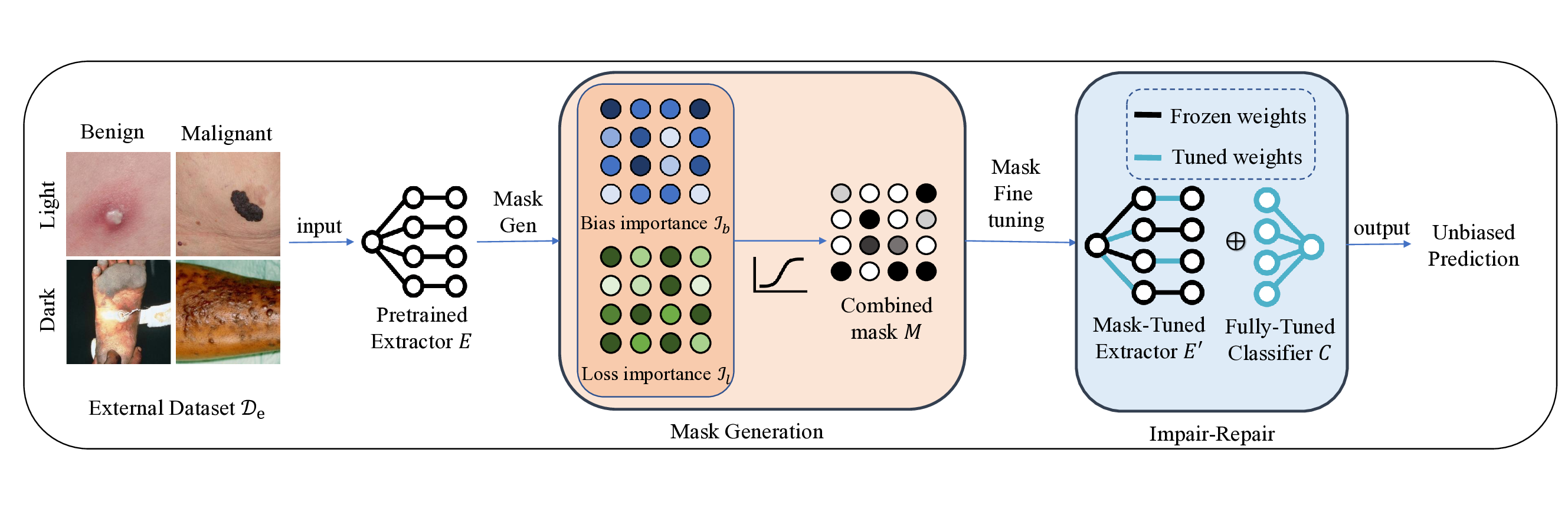
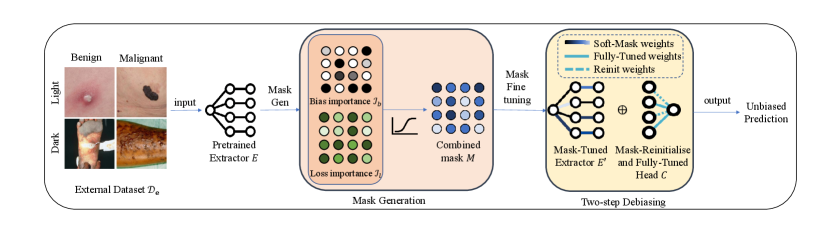
We propose an efficient and effective debiasing framework, called Soft-Mask Weight Fine-Tuning (SWiFT). Unlike pre- or in-processing debiasing methods, SWiFT requires only a few epochs of fine-tuning instead of full model retraining. Furthermore, our approach uses only a small external dataset (in our experimental work, no more than $25\%$ of the original training set size), thus eliminating the need for extensive or often inaccessible training data – a common practical limitation. Compared to post-processing methods, SWiFT effectively preserves core features for prediction while removing bias features, yielding superior debiasing and discriminative performance across diverse metrics. As illustrated in Figure 2, SWiFT operates under the following procedure: given a pre-trained biased model, the first step is to generate a parameter-wise soft-mask, which quantifies each network parameter’s relative contribution to bias versus prediction performance. During debiasing, this soft-mask constrains gradient flows during backpropagation, ensuring minimal changes to parameters important for prediction and preserving core features. Next, SWiFT employs a two-step debiasing strategy: firstly, it fine-tunes the feature extractor parameters with gradient flows modulated by the soft-mask to remove bias from features; secondly, to eliminate bias from incorrect feature compositions within the classification head, we partially re-initialize its parameters to erase the weights of previously learned, bias features. The entire head is then fine-tuned to learn a robust feature combination with only the core features. Our main contributions are summarized as follows:

$\bullet$
We propose a novel debiasing framework capable of mitigating bias and improving fairness and generalizability, without compromising model discriminative performance. Our framework circumvents expensive full model retraining and original training data access requirements.
$\bullet$
A soft-mask generation technique that quantitatively measures network parameter contributions towards bias features vs. core features, enabling targeted debiasing through differentiated parameter updates. To the best of our knowledge, our work is the first to employ model parameter soft-masking to the debiasing task.
$\bullet$
We propose a two-step fine-tuning strategy that is model-agnostic and effectively removes model bias through only a few epochs of fine-tuning on a small external dataset.
$\bullet$
Experiments on four out-of-distribution (OOD) dermatological disease and two OOD chest X-ray datasets demonstrate that SWiFT outperforms nine state-of-the-art (SOTA) methods, with respect to both fairness and discriminative capabilities.

A preliminary version of this work, named BMFT (Xue et al., 2024), was presented at the MICCAI FAIMI Workshop 2024. In this journal extension we include: i) four methodological modifications that improve generalization, robustness, and effectiveness over our previous method. First, we introduce a novel soft-mask generation module that enables more adaptive and fine-grained model updates. Unlike the previous hard-mask, which optimizes parameters based on a predefined threshold and freezes others, soft-mask does not fully block parameters and keeps most parameters trainable. This provides the network with greater capacity to update parameters towards core features and removes the need for exhaustive threshold tuning. Second, we propose a partial classification head re-initialization strategy. It preserves well-learned core features that facilitates feature re-combination with faster convergence speed. Third, we improve the loss function with dynamic balancing between classification loss and fairness constraints, enhancing adaptability across different tasks and datasets. Finally, we extend SWiFT to handle multi-attribute bias removal scenarios. Modifications are accompanied with new experiments which demonstrate the respective improvements compared to BMFT and other baselines. ii) New experimental validation. We perform new experiments with 5-fold cross-validation, introduce new experimental domains with chest-xray datasets, and evaluate SWiFT on two additional network architectures, EfficientNet-B3 and DenseNet-121, to validate its robustness and generalization to different scenarios. Lastly, we conduct comprehensive ablation studies to analyze the contribution of each module, the role of the external dataset, and the sensitivity to hyperparameters. iii) Additional experiments analysis: we provide an in-depth analysis of the experimental results with additional quantitative evaluations and qualitative insights through Class Activation Maps (CAMs).

2 Related Work

In this section, we firstly review fairness challenges in medical imaging classification tasks. We next provide a brief survey on recent debiasing methods proposed to tackle these challenges, and finally discuss existing mask fine-tuning techniques, highlighting how our soft-mask-based debiasing approach builds upon and extends previous work.

2.1 Bias and Fairness in Medical Imaging

Bias and fairness are widely reported in medical imaging analysis (Luo et al., 2024; Wang et al., 2017; Zhang et al., 2022). Bias in ML systems leads to unfair decision-making, thus undermining model fairness. Bias can arise from various sources, including label noise, data imbalance, and spurious correlations (Mehrabi et al., 2021). A critical concern is bias amplification, where biases in the training data are amplified by model predictions during deployment (Dutt et al., 2024). This not only compromises model fairness and generalization, but also risks exacerbating social discrimination (Mehrabi et al., 2021). Achieving fairness in medical AI is thus both a technical challenge and an ethical imperative. Fairness in ML systems is often measured through group fairness (Mehrabi et al., 2021), which aims to ensure similar average outcomes across demographic groups. Common metrics for group fairness include statistical parity difference (SPD)(Marcinkevics et al., 2022), equal opportunity (EO) (Hardt et al., 2016), and equalized odds (EOdds)(Hardt et al., 2016). However, optimizing for group fairness can lead to a reduction in individual fairness, often resulting in decreased prediction accuracy (Zietlow et al., 2022). Therefore, debiasing is inevitably a multi-objective challenge that seeks to simultaneously achieve good discriminative performance and good fairness.

2.2 Debiasing Methods

Existing bias mitigation methods in medical imaging can be categorized into three groups: pre-processing, in-processing, and post-processing. Pre-processing methods debias the training data before the training process. Current approaches include either transforming data representations to eliminate correlations between feature representations and sensitive attributes (Zhang et al., 2022), (Yuan et al., 2023) or augmenting data distributions to equalize the training distribution across different demographic groups (Oguguo et al., 2023), (Zietlow et al., 2022). Pre-processing methods often require extensive data processing efforts, and commonly used data augmentation strategies (e.g. color permutation (Park et al., 2022)) may not be suitable for certain medical modalities (e.g. CT scans). In-processing methods address fairness during the model training process, typically by modifying the loss function to regularize the model and mitigate bias. For example, Zafar et al. (2017) incorporate bias-specific regularization terms in the loss function. Jung et al. (2023) employed a classwise distributionally robust optimization framework to mitigate group disparities. Zhao et al. (2022) used adversarial learning to remove sensitive information. In-processing methods cannot explicitly protect the underrepresented group when enforcing the fairness constraints, often resulting in accuracy drops for both groups. Additionally, both pre- and in-processing methods necessitate access to the original training data and require model retraining, limiting their efficiency in real-world scenarios.Post-processing techniques, in contrast, are performed after training and achieve fairness by modifying model predictions or parameters. Oguguo et al. (2023) achieve fairness by flipping unfavorable predictions of the minority group on instances where the model exhibits high uncertainty. Marcinkevics et al. (2022) and Wu et al. (2022) mitigate unfairness by pruning parameters based on their contribution to bias. However, debiasing by simply changing specific sample predictions or removing neurons may be problematic. Such approaches can be unfair to certain individuals and may cause the model to lose information about core features, leading to unsatisfactory trade-offs between accuracy and fairness (Chen et al., 2024).

To address the outlined challenges, our method applies fine-tuning over only a few epochs using a small external dataset, without the need to modify the data or retrain the model. Our approach considers both prediction and bias constraints by estimating model parameter contributions towards core and bias features, resulting in high overall accuracy and fairness.

2.3 Mask Fine-tuning

Fine-tuning a model that has been pre-trained on a large dataset towards a specific downstream task is common practice in machine learning (Ben Zaken et al., 2022). Leveraging the knowledge embedded in pre-trained models often enables downstream tasks to be learned with significantly less data compared to training from scratch. Mask fine-tuning methods are a family of techniques designed to improve the fine-tuning process by controlling parameter updates according to their importance on the objective. Current approaches, such as Parameter Efficient Fine Tuning (Ben Zaken et al., 2022; Dutt et al., 2024), employ the binary-mask (hard-mask) to select a subset of parameters to update while freezing the rest. Hard-masks typically require extensive hyperparameter tuning to determine the optimal selection rate of parameters for fine-tuning versus freezing (Wu et al., 2022; Dutt et al., 2024). Moreover, we note that hard-masks provide only a relatively blunt tool to differentiate the contributions of specific parameters towards the objective. Konishi et al. (2023) proposed the use of soft-masks in continual learning tasks, which are flexible and efficient. We investigate a soft-mask fine-tuning strategy to mitigate bias and improve fairness. Overall, our method demonstrates the superiority of soft-mask over binary-mask in terms of both fairness and accuracy.

3 Methodology

The core idea of our method, see Figure 2, is to discriminately control model parameter updates based on their relative individual contributions to both bias and predictive performance. Key to our method is the soft-mask generation, which regulates model parameter updates during debiasing. The debiasing process consists of a two-step fine-tuning strategy that uses the soft-mask to debias the model feature extractor and the classification head, sequentially. Before we proceed to detail our method we begin with preliminaries.

3.1 Preliminaries

Problem Formulation We study a supervised image classification problem where we will impose fairness considerations. We define disjoint training, validation, and test datasets such that $\mathcal{D}_{\mathrm{train}}\cup\mathcal{D}_{\mathrm{valid}}\cup\mathcal{D}_{\mathrm{test}}=\{\mathbf{x}_{i},y_{i},a_{i}\}$ , where $\mathbf{x}_{i}$ denotes input image $i$ with class label $y_{i}$ , and $a_{i}$ is a 1D binary vector that represents the presence or absence of sensitive attributes for sample $i$ (e.g. skin tone, gender, age). In this work we assume binary prediction targets and sensitive attributes (i.e. $y_{i},a_{i}\in\{0,1\}$ ). Let $f_{\theta}(\cdot)$ denote a biased (i.e. lacking in group fairness) model parameterized by $\theta$ . We assume a decomposable model consisting of a feature extractor $E(\cdot)$ and a classification head $C(\cdot)$ , which is pre-trained on the original training data $\mathcal{D}_{\mathrm{train}}$ .

Our goal is to debias $f_{\theta}(\cdot)$ , as measured by existing fairness metrics such as Statistical Parity Difference (SPD) (Dwork et al., 2012) and Equalised Odds (EOdds) (Hardt et al., 2016), by fine-tuning for only a few epochs with the external dataset $\mathcal{D}_{e}$ . With this procedure, we aim to enhance the model’s reliance on core features and further improve its generalizability, which can be evidenced by improved AUC on various OOD test datasets $\mathcal{D}_{\mathrm{test}}$ that share the same sensitive attribute $a_{i}$ .

External Dataset Preparation The external dataset can be readily constructed from labeled data that shares the same task categories as the training data $\mathcal{D}_{\mathrm{train}}$ . As a proof of concept, our experimental work constructs $\mathcal{D}_{e}$ from each task’s respective validation dataset. The external dataset must contain samples both with and without biased features. This enables the debiasing method to accurately identify biased representations within the pre-trained model and subsequently mitigate them during model fine-tuning. To avoid introducing new sources of biases (i.e., group attribution bias, label bias) from $\mathcal{D}_{e}$ , we employ common group-balancing strategies (Zhang et al., 2022; Mao et al., 2023) to prepare our external dataset. Specifically, we keep all data from the smallest attribute group, and subsample the data from the other group to the same size and classification label ratios. Therefore, our method does not require the same label or sensitive distributions between the final external dataset and the training/test data; in fact, it leverages the balanced distribution across sensitive groups within $\mathcal{D}_{e}$ to effectively debias the model.

3.2 Soft-Mask Generation

Model parameters contribute non-uniformly to bias features that affect fairness and core features that drive predictive performance (Wu et al., 2022; Dutt et al., 2024). Therefore, parameters require differentiated adjustment during debiasing. To address this, we define a soft-mask that assigns larger updates to parameters contributing primarily to bias and smaller updates that preserve features crucial for prediction. In this way, the core features are retained while bias is mitigated. To construct our mask, we calculate the respective per-parameter importance according to relevant prediction and bias functions.

Prediction function We adopt Weighted Binary Cross Entropy (WBCE (Xue et al., 2024)), which is a robust cross-entropy term w.r.t. class imbalance – a common trait of medical imaging datasets (Bevan and Atapour-Abarghouei, 2022; Puyol-Antón et al., 2021):

$\mathcal{L}_{\mathrm{WBCE}}=\sum_{i}\left(-\frac{N_{n}}{N_{n}+N_{p}}\mathbf{y}_{i}\log(p_{i})-\frac{N_{p}}{N_{n}+N_{p}}(1-\mathbf{y}_{i})\log(1-p_{i})\right).$

(1)

Bias function We use the differentiable proxy of EOdds (Hardt et al., 2016):

\mathcal{B}(f_{\theta},\mathcal{D}_{e})=tpr+fpr,

(2)

where

$tpr=\left|\frac{\sum_{i}(1\!-\!a_{i})y_{i}\log(f_{\theta}(x_{i}))}{\sum_{i}(1\!-\!a_{i})y_{i}}\!-\!\frac{\sum_{i}a_{i}y_{i}\log(f_{\theta}(x_{i}))}{\sum_{i}a_{i}y_{i}}\right|\raisebox{-8.61108pt}{,}$

(3)

$fpr=\left|\frac{\sum_{i}\!(1\!-\!a_{i})(1\!-\!y_{i})\log(f_{\theta}(x_{i}))}{\sum_{i}(1\!-\!a_{i})(1\!-\!y_{i})}\!-\!\frac{\sum_{i}a_{i}(1\!-\!y_{i})\log(f_{\theta}(x_{i}))}{\sum_{i}a_{i}(1\!-\!y_{i})}\right|\raisebox{-8.61108pt}{,}$

(4)

where $f_{\theta}(x_{i})$ provides a predictive probability for sample $x_{i}$ under a binary classification task. EOdds requires that a model’s predictions are independent of sensitive group memberships with different sensitive groups having the same false positive rates and true positive rates. The EOdds is defined for binary sensitive attributes. To extend its application to multi-attribute scenarios, we employ a targeted optimization strategy. Specifically, we first identify the attribute groups with the highest and lowest Area Under the Curve (AUC) scores to serve as proxies for the most advantaged and disadvantaged groups. We then apply the EOdds bias function to this pair of groups. The effectiveness of this approach is evaluated in Section 5.1.3.

Estimating parameter importance Previous work (Foster et al., 2024; Kirkpatrick et al., 2017) has demonstrated that the parameter importance towards an objective function can be effectively calculated using the Fisher Information Matrix (FIM). Given a probability density function (PDF) $p(\mathcal{D}_{e}|\theta)$ , the FIM over dataset $\mathcal{D}_{e}$ is defined by:

\small\mathcal{I}(\theta,\mathcal{D}_{e})=-\mathbb{E}_{\mathcal{D}_{e}}\bigtriangledown^{2}_{\theta}\log p(\mathcal{D}_{e}|\theta).

(5)

The full FIM is an $n\times n$ matrix, typically making the calculation computationally expensive. Thus we follow Foster et al. (2024); Kirkpatrick et al. (2017) and further approximate the FIM using its diagonal values, as given by:

\small\mathcal{I}(\theta,\mathcal{D}_{e})=-\mathbb{E}\!\left[\!\left(\frac{\partial\log p(\mathcal{D}_{e}|\theta)}{\partial\theta}\!\right)\!\left(\!\frac{\partial\log p(\mathcal{D}_{e}|\theta)}{\partial\theta}\!\right)^{\top}\!\right]\raisebox{-7.74997pt}{.}

(6)

Given a pre-trained model $f_{\theta}$ and the external dataset $\mathcal{D}_{e}$ , the log-likelihoods of the prediction PDF and bias PDF are simply the negative of the WBCE function and bias function in Eq. (2), respectively. Therefore, the parameter importance, in terms of influencing prediction accuracy, is given by:

\small\mathcal{I}_{l}(\theta,\mathcal{D}_{e})=\mathbb{E}\!\left[\!\left(\frac{\partial\mathcal{L}_{\mathrm{WBCE}}(\mathcal{D}_{e}|\theta)}{\partial\theta}\!\right)\!\left(\!\frac{\partial\mathcal{L}_{\mathrm{WBCE}}(\mathcal{D}_{e}|\theta)}{\partial\theta}\!\right)^{\top}\!\right].

(7)

Whereas, the parameter importance in terms of influencing model bias can be computed by:

\small\mathcal{I}_{b}(\theta,\mathcal{D}_{e})=\mathbb{E}\!\left[\!\left(\frac{\partial\mathcal{B}(\mathcal{D}_{e}|\theta)}{\partial\theta}\!\right)\!\left(\!\frac{\partial\mathcal{B}(\mathcal{D}_{e}|\theta)}{\partial\theta}\!\right)^{\top}\!\right].

(8)

Mask Construction Having defined estimates for parameter importance, with respect to both predictive accuracy and bias, we design our weight soft-mask according to the relative ratio between the introduced importance terms. We denote each continuous scalar element of the weight mask as $M_{i}$ , where $i$ is the weight index. An element of the mask is defined as:

\mathcal{M}_{i}=\left|\mathrm{\tanh}\left(\frac{\text{Norm}(\mathcal{I}_{i,b})}{\text{Norm}(\mathcal{I}_{i,l})}\right)\right|,

(9)

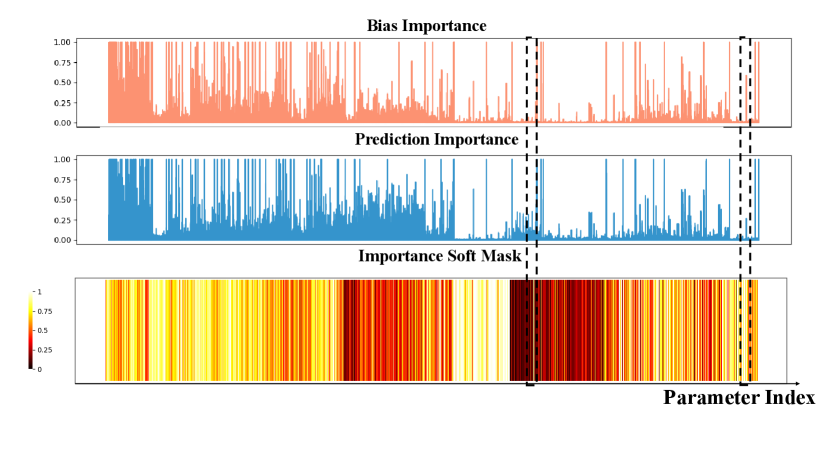
where $\mathcal{I}_{i,l}$ and $\mathcal{I}_{i,b}$ are the $i$ -th diagonal elements of the FIMs in Eq. (7) and Eq. (8), respectively, and $\text{Norm}(\cdot)$ denotes min–max normalization. Normalizing gradients with respect to each network layer helps us avoid discrepancies due to large differences in gradient magnitude. The components of Eq. (9) serve specific purposes. First, since the two importance terms may have different numerical scales, we normalize them with respect to each network layer. This ensures their ratio provides a meaningful measure of a parameter’s relative contribution to bias versus prediction. Our choice is empirically validated in Section 5.2.2, where we show that min-max normalization yields superior results compared to z-score normalization for this task. Second, the raw ratio of these terms is unbounded. We therefore apply the hyperbolic tangent (tanh) function to introduce non-linearity and map the unbounded input to a finite interval. Finally, since the magnitude of the gradient rather than its sign indicates a strong importance (i.e., values near $-1$ and $+1$ are both significant), we take the absolute value. This ensures that each mask element $M_{i}$ lies within the range $[0,1]$ . Due to this construction, a higher value of $M_{i}$ represents a weight that is predicted to have larger importance for attribute bias and a less significant impact on predictive accuracy. The parameters with higher mask values will constitute the significant updates during fine-tuning. In the following section, we provide a strategy that uses this signal to remove the detrimental influence of model bias, while retaining information embedded in core features. An illustrative example of bias importance, prediction importance, and the resulting soft-mask is provided in Figure 3.

3.3 Two-Step Fine-Tuning

Model bias typically originates from two key sources (Le et al., 2023): (1) the entanglement between harmful bias features (typically spurious or irrelevant) and useful core (causal) features, within the feature extractor; and (2) the incorrect composition of representations in the classification head (i.e., bias features are highly weighted in the classification head, causing the final predictions to rely on bias). Our method establishes a two-step fine-tuning process to address the two key sources sequentially.

Feature Extractor: Soft-Mask Fine-Tuning Core features that exist in pre-trained models are often entangled with bias features (Le et al., 2023). To address this, our first fine-tuning step debiases the feature extractor $E(\cdot)$ while keeping the classification head $C(\cdot)$ frozen. The goal of this fine-tuning process is two-fold: to remove bias features that may compromise fairness and to preserve core features essential for accurate prediction. We achieve this goal by optimizing the feature extractor with a bias-specific loss function, while constraining updates of prediction-important parameters. Specifically, we fine-tune the feature extractor on $\mathcal{D}_{e}$ using a loss function that combines the WBCE loss $\mathcal{L}_{\mathrm{WBCE}}$ with a fairness constraint (Eq. 2):

\small\mathcal{L}=\beta\mathcal{L}_{\mathrm{WBCE}}(f_{\theta},\mathcal{D}_{e})+(1-\beta)\mathcal{B}(f_{\theta},\mathcal{D}_{e}),

(10)

where $\mathcal{B}(f_{\theta},\mathcal{D}_{e})$ represents our objective relating to reducing bias. The hyperparameter $\beta\in[0,1]$ explicitly balances the prediction accuracy and fairness objectives. $\beta$ is fixed within each step of our two-step fine-tuning pipeline, but may differ between steps. In this first step, we set $\beta$ to a small value $\epsilon$ to prioritize feature debiasing during feature extractor fine-tuning. During the backward pass, we modify the gradients of all parameters in the feature extractor using the soft-mask. This mask modulates each parameter’s update according to its relative bias-prediction importance ratio:

g_{i}^{\prime}=\mathcal{M}_{i}g_{i},

(11)

where $g_{i}$ and $g_{i}^{\prime}$ represent the original and modified gradients of the $i^{\text{th}}$ model parameter $\theta_{i}$ , respectively. This soft-masked gradient adjustment ensures that parameters critical for prediction accuracy are updated less aggressively, while bias-related parameters are targeted for more significant modification.

Classification Head: Re-initialization and Fine-tuning The previous fine-tuning step reduces bias originating from core and bias feature entanglement in the feature extractor. We introduce here our second step to re-combine debiased features within the classification head. Since the feature extractor already contains well-learned representations, fine-tuning the classification head is known to converge very quickly, often before model parameters can be sufficiently updated towards new or modified objectives (Li et al., 2020). In our setting, this results in classification decisions remaining heavily influenced by original features rather than debiased features (Zhang et al., 2017), limiting fairness and accuracy gains. To address this issue, we propose parameter re-initialization as an effective strategy to push significant and meaningful updates in the classification head, thus promoting the learning of correct combinations of debiased core features (Ramkumar et al., 2024; Kirichenko et al., 2023).

Recent works (Xue et al., 2024; Mao et al., 2023) suggest strategies that re-initialize the entire classification head $C(\cdot)$ . This risks losing all discriminative ability of the pre-trained model where recovery would require retraining, typically not achievable by small epoch counts. Therefore, we alternatively re-initialize only a portion of parameters, based on the mask calculated using Eq. 9. Parameters with high mask values, indicating their disproportionately strong influence on the bias features, are re-initialized to zero. This zero re-initialization strategy is inspired by Le et al. (2023) where it was shown that, for an unbiased model trained on a balanced dataset, most classification head parameters converge to zero. In our setting, re-initializing bias-important parameters to zero facilitates rapid convergence towards an unbiased state where it is understood that subsets of parameters can be initialized to zero without causing training degeneracy (Zhao et al., 2022). The re-initialization threshold $\gamma$ is determined by the mean value of the mask calculated on the classification head parameters. The partial re-initialization process is shown as Eq. (12).

\small\theta_{i}^{\prime}=\left\{\begin{array}[]{ll}0,&\text{if}\ \ \mathcal{M}_{\theta_{i}}\geq\gamma\\ \theta_{i},&\text{otherwise},\\ \end{array}\right.

(12)

Finally, we fine-tune the re-initialized classification head while keeping the feature extractor frozen, using the Eq. (10) objective. Different from the first step, we typically set a much larger hyperparameter value of $\beta$ = $1-\epsilon$ at this stage, to place more emphasis on retaining the model’s discriminative capability.

4 Experimental Setup

We next detail our experimental work where the proposed method is validated under two inference tasks: skin lesion classification and chest X-ray classification. In the following subsections we introduce the considered tasks, provide implementation details and evaluation settings.

4.1 Datasets and Pre-processing

In both tasks, we perform a five-fold cross-validation to evidence the efficacy and statistical significance of our method. The original dataset is split into training set and validation set with an $80{:}20$ ratio, ensuring no overlap. The model is pre-trained on the training dataset and was debiased via fine-tuning on the external dataset (i.e. constructed from the validation dataset). The debiased model is then tested on various out-of-distribution (OOD) test datasets, which may exhibit distributional shifts in both disease labels and sensitive attributes, relative to the training data.

4.1.1 Skin Lesion Classification

We use the International Skin Imaging Collaboration (ISIC) Challenge Dataset for pre-training and fine-tuning. We treat “melanoma” as the negative class and all other lesions as the positive class. We combine 2017 (Codella et al., 2018), 2018 (Codella et al., 2019), 2019 (Tschandl et al., 2018; Hernández-Pérez et al., 2024) and 2020 (Rotemberg et al., 2021) ISIC challenge data, and remove duplicate images across different years, totaling 56,863 images. Among these, 45,489 images are used for training, while 11,374 images are reserved as the validation dataset in each fold. We consider two sensitive attributes: skin tone and gender. We maintain the same skin tone annotation as Bevan and Atapour-Abarghouei (2022) for training data. To build the group-balanced external dataset $\mathcal{D}_{e}$ , we select c. 3,600 images for skin tone and c. 11,000 for gender. All images are pre-processed with center-cropping and resizing to size $256{\times}256$ .

For testing, our study employs four OOD datasets with skin images for melanoma detection. Fitzpatrick-17k (Groh et al., 2021) contains 16,577 images across six skin tone levels, which we group into light (1-3) and dark (4-6) categories. DDI (Daneshjou et al., 2022) offers 656 images with skin tone annotations. Interactive Atlas of Dermoscopy (Atlas) (Lio and Nghiem, 2004) and PAD-UFES-20 (Pacheco et al., 2020) contain gender labels with 1,011 images and 2,298 images, respectively.

4.1.2 Chest X-ray Classification

We train a model on the large-scale chest X-ray dataset MIMIC-CXR (Johnson et al., 2019). We use only frontal view images, and resize to $224{\times}224$ pixels. We consider a binary classification problem of “pneumothorax” and “No Findings”, where these classes are treated as positive and negative, respectively. The problem definition is consistent with previous chest X-ray fairness research (Seyyed-Kalantari et al., 2020; Zhang et al., 2022). In each cross-validation fold, 61,502 images are randomly selected for training, while the remaining 15,376 images are used as the validation set. We focus on two sensitive attributes (gender and age) since the groups of these attributes are previously shown to have disparate classification outcomes (Wang et al., 2017; Zhang et al., 2022). For age, we categorize individuals into a younger group ( $\leq 65$ years old) and an older group ( $>65$ years old), following established definitions in (Singh and Bajorek, 2014). 14,950 images for gender and 10,360 images for age are selected to build the external dataset $\mathcal{D}_{e}$ for fine-tuning.

We evaluate our method on two OOD datasets; Chexpert (Irvin et al., 2019) and Chest-Xray8 (NIH) (Wang et al., 2017). We select CXRs with “Pneumothorax”, “No Findings” labels from Chexpert and NIH, which are 21,040 and 10,815 images, respectively. Both datasets include sensitive attributes: gender (Female and Male) and age (0–80), making them suitable for assessment of fairness and accuracy metrics.

4.2 Implementation

We conduct experiments in PyTorch using one NVIDIA A100 40GB GPU. For skin lesion classification, We apply ImageNet-pretrained ResNet50 and Efficient B3 as the model backbone. The models are trained for 200 epochs using an SGD optimizer with a batch size 128 and a learning rate 1e-4. For chest X-ray classification, we choose ImageNet-pretrained ResNet50 and DenseNet-121 as the backbone. The models are trained for 100 epochs using an Adam optimizer with a batch size of 128 and a learning rate of 1e-4. The pre-training process for both tasks follows previous fairness research (Bevan and Atapour-Abarghouei, 2022; Mao et al., 2023; Zhang et al., 2022; Marcinkevics et al., 2022). For debiasing the model, we fine-tune the skin pre-trained model and the chest X-ray pre-trained model for an additional 20, 10 epochs, respectively, which are 10% of the initial training duration. Equal epoch counts are used for both stages of two-step fine-tuning. The fine-tuning process shares the same optimizer and batch size as the training process. Data augmentation was applied in both training and fine-tuning, which includes random flipping, random transpose, and $z$ -score normalization.

4.3 Comparison Method and Evaluation Metrics

We compare our methods with nine recent SOTA models. The model pre-trained on the training dataset $\mathcal{D}_{\mathrm{train}}$ is our basic Baseline. FullFT-RW (Zhang et al., 2022) fine-tunes the pre-trained model on the group-balanced external data $\mathcal{D}_{e}$ using only the prediction loss. FullFT-Reg (Cherepanova et al., 2021) fine-tunes the pre-trained model on the non group-balanced dataset $\mathcal{D}_{val}$ using a combination of prediction loss and fairness constraints in the form of Eq. (10). FullFT-FDR (Le et al., 2023) combines data balancing and fairness constraints, fine-tuning all parameters on the dataset $\mathcal{D}_{e}$ with the loss function specified in Eq. (10). LLFT (Mao et al., 2023) fine-tunes only the last layer of a deep classification model to promote fairness. Similarly, DiffGda (Marcinkevics et al., 2022) fine-tunes on an external dataset, using a bias-aware loss function to steer network optimization. FairPrune (Wu et al., 2022) improves fairness by pruning parameters based on weight saliency. DiffPrune (Marcinkevics et al., 2022) prunes parameters based on their contributions to bias. BMFT (Xue et al., 2024) is a hard-mask based fine-tuning method for debiasing (our work, prior to SWiFT).

To evaluate the discriminative performance of different models, we use the area under the curve (AUC) as a primary performance metric, and statistical parity difference (SPD) ((Daneshjou et al., 2022)) and equalized odds (EOdds) ((Hardt et al., 2016)) as fairness metrics, similar to previous work (Dutt et al., 2024; Chen et al., 2024; Wu et al., 2022).

4.4 Hyperparameter Validation

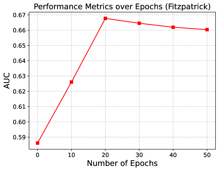
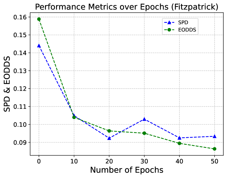
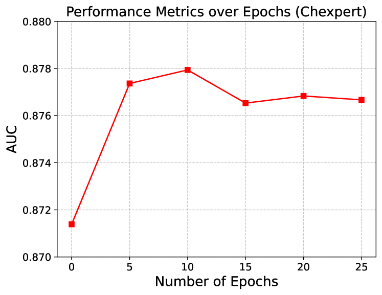
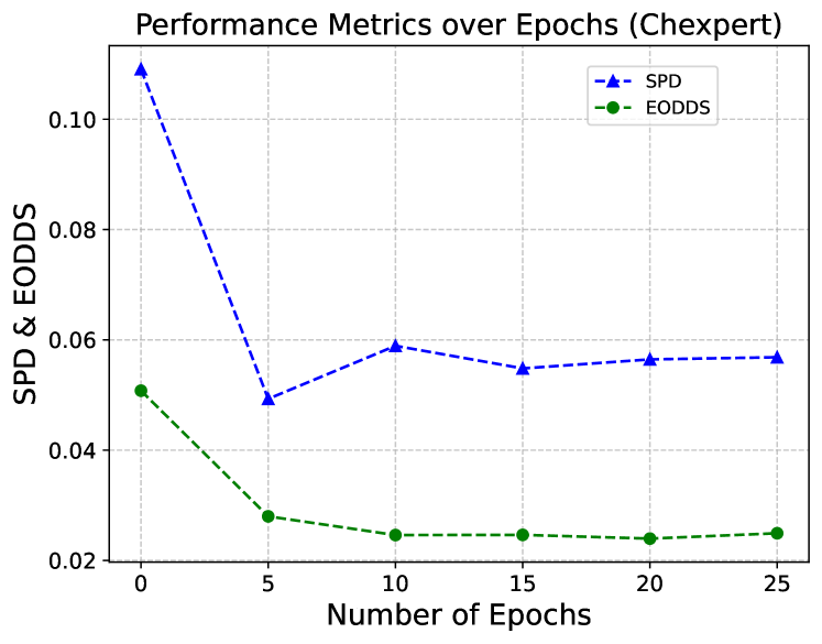
Determining the optimal number of fine-tuning epochs is important for effectively balancing computational efficiency and debiasing performance for our experimental work. We empirically explore the impact of the number of fine-tuning epochs on skin tone debiasing in skin lesion classification and age debiasing in the chest X-ray classification. The results are shown in Figure 4. The $0^{th}$ epoch is the pre-trained baseline model. As we can see, both prediction and fairness metrics improve even with only $5\%$ of the original training epochs (i.e., 10 epochs for skin tone debiasing, and 5 epochs for age debiasing), and become steady after $10\%$ of the original training epochs. The debiasing time increases linearly with the number of fine-tuning epochs. Moreover, the AUC tends to decrease as the number of epochs increases, likely due to overfitting during fine-tuning on the small dataset. Based on these findings, we select $10\%$ of the training epochs (i.e., $20$ epochs for skin tone debiasing and $10$ epochs for age debiasing) for subsequent evaluation and comparison with other methods.

5 Results

We report performance across our investigated experimental scenarios where we aim to answer our primary question: can model fairness be improved, and discriminative performance maintained, under data and compute frugal regimes? Further, we conjecture that debiased models should generalize effectively across different data distributions and sensitive attributes. Towards exploring this point we evaluate the fairness and predictive accuracy of our approach on several OOD test datasets, each with distinct sensitive attributes.

5.1 Comparison with SOTA Debiasing Methods

5.1.1 Quantitative Results

Table 1: Comparison of debiasing methods on skin tone and gender. ResNet-50 model pre-trained on ISIC dataset (MEAN

\pm

STD). Results are consistently denoted best and second best for all Tables.

Attr.MethodsFitzpatrick-17kDDI AUC $\uparrow$ SPD $\downarrow$ EOdds $\downarrow$ AUC $\uparrow$ SPD $\downarrow$ EOdds $\downarrow$ Skin ToneBaseline0.586 $\pm$ 0.0080.144 $\pm$ 0.0080.159 $\pm$ 0.0070.601 $\pm$ 0.0050.101 $\pm$ 0.0200.113 $\pm$ 0.025FullFT-RW (Zhang et al., 2022)0.586 $\pm$ 0.0090.146 $\pm$ 0.0130.160 $\pm$ 0.0110.592 $\pm$ 0.0080.126 $\pm$ 0.0200.141 $\pm$ 0.022FullFT-Reg (Cherepanova et al., 2021)0.589 $\pm$ 0.0060.118 $\pm$ 0.0150.131 $\pm$ 0.0120.587 $\pm$ 0.0060.116 $\pm$ 0.0420.126 $\pm$ 0.034FullFT-FDR (Le et al., 2023)0.587 $\pm$ 0.0130.110 $\pm$ 0.0150.123 $\pm$ 0.0120.580 $\pm$ 0.0080.128 $\pm$ 0.0400.128 $\pm$ 0.038LLFT (Mao et al., 2023)0.571 $\pm$ 0.0160.097 $\pm$ 0.0160.113 $\pm$ 0.0140.590 $\pm$ 0.0130.069 $\pm$ 0.0370.088 $\pm$ 0.043DiffGda (Marcinkevics et al., 2022)0.586 $\pm$ 0.0080.144 $\pm$ 0.0060.156 $\pm$ 0.0080.600 $\pm$ 0.0050.106 $\pm$ 0.0150.116 $\pm$ 0.017FairPrune (Wu et al., 2022)0.560 $\pm$ 0.0070.101 $\pm$ 0.0120.120 $\pm$ 0.0150.564 $\pm$ 0.0280.102 $\pm$ 0.0460.119 $\pm$ 0.055DiffPrune (Marcinkevics et al., 2022)0.589 $\pm$ 0.0080.116 $\pm$ 0.0060.127 $\pm$ 0.0060.598 $\pm$ 0.0040.086 $\pm$ 0.0100.097 $\pm$ 0.009BMFT (Xue et al., 2024)0.651 $\pm$ 0.0120.119 $\pm$ 0.0130.114 $\pm$ 0.0120.610 $\pm$ 0.0150.099 $\pm$ 0.0150.094 $\pm$ 0.020SWiFT (Ours)0.668 $\pm$ 0.0130.092 $\pm$ 0.0280.096 $\pm$ 0.0260.625 $\pm$ 0.0100.063 $\pm$ 0.0300.064 $\pm$ 0.036AtlasPAD AUC $\uparrow$ SPD $\downarrow$ EOdds $\downarrow$ AUC $\uparrow$ SPD $\downarrow$ EOdds $\downarrow$ GenderBaseline0.788 $\pm$ 0.0050.026 $\pm$ 0.0080.031 $\pm$ 0.0100.717 $\pm$ 0.0090.009 $\pm$ 0.0050.036 $\pm$ 0.014FullFT-RW (Zhang et al., 2022)0.788 $\pm$ 0.0060.021 $\pm$ 0.0070.022 $\pm$ 0.0060.718 $\pm$ 0.0080.011 $\pm$ 0.0080.035 $\pm$ 0.020FullFT-Reg (Cherepanova et al., 2021)0.780 $\pm$ 0.0050.024 $\pm$ 0.0110.041 $\pm$ 0.0180.703 $\pm$ 0.0170.018 $\pm$ 0.0050.036 $\pm$ 0.030FullFT-FDR (Le et al., 2023)0.779 $\pm$ 0.0060.030 $\pm$ 0.0110.040 $\pm$ 0.0190.702 $\pm$ 0.0180.012 $\pm$ 0.0070.051 $\pm$ 0.031LLFT (Mao et al., 2023)0.774 $\pm$ 0.0040.019 $\pm$ 0.0060.024 $\pm$ 0.0030.701 $\pm$ 0.0080.012 $\pm$ 0.0060.031 $\pm$ 0.018DiffGda (Marcinkevics et al., 2022)0.786 $\pm$ 0.0050.030 $\pm$ 0.0130.035 $\pm$ 0.0180.723 $\pm$ 0.0080.011 $\pm$ 0.0080.022 $\pm$ 0.014FairPrune (Wu et al., 2022)0.691 $\pm$ 0.0510.016 $\pm$ 0.0100.018 $\pm$ 0.0100.619 $\pm$ 0.0570.018 $\pm$ 0.0140.055 $\pm$ 0.019DiffPrune (Marcinkevics et al., 2022)0.768 $\pm$ 0.0080.006 $\pm$ 0.0040.012 $\pm$ 0.0080.719 $\pm$ 0.0100.010 $\pm$ 0.0130.033 $\pm$ 0.015BMFT (Xue et al., 2024)0.787 $\pm$ 0.0050.005 $\pm$ 0.0050.014 $\pm$ 0.0060.727 $\pm$ 0.0110.005 $\pm$ 0.0050.032 $\pm$ 0.032SWiFT (Ours)0.789 $\pm$ 0.0050.012 $\pm$ 0.0070.010 $\pm$ 0.0060.728 $\pm$ 0.0090.006 $\pm$ 0.0050.031 $\pm$ 0.004

Table 2: Comparison of debiasing methods on skin tone and gender. Efficient-B3 model pre-trained on ISIC dataset.

Attr.MethodsFitzpatrick-17kDDI AUC $\uparrow$ SPD $\downarrow$ EOdds $\downarrow$ AUC $\uparrow$ SPD $\downarrow$ EOdds $\downarrow$ Skin ToneBaseline0.625 $\pm$ 0.0080.039 $\pm$ 0.0050.047 $\pm$ 0.0070.600 $\pm$ 0.0080.082 $\pm$ 0.0080.101 $\pm$ 0.014FullFT-RW (Zhang et al., 2022)0.625 $\pm$ 0.0090.049 $\pm$ 0.0070.053 $\pm$ 0.0120.600 $\pm$ 0.0090.112 $\pm$ 0.0190.121 $\pm$ 0.022FullFT-Reg (Cherepanova et al., 2021)0.610 $\pm$ 0.0060.029 $\pm$ 0.0090.032 $\pm$ 0.0120.594 $\pm$ 0.0050.089 $\pm$ 0.0040.119 $\pm$ 0.007FullFT-FDR (Le et al., 2023)0.616 $\pm$ 0.0080.030 $\pm$ 0.0130.029 $\pm$ 0.0150.603 $\pm$ 0.0050.080 $\pm$ 0.0150.109 $\pm$ 0.022LLFT (Mao et al., 2023)0.612 $\pm$ 0.0080.014 $\pm$ 0.0090.028 $\pm$ 0.0090.596 $\pm$ 0.0120.029 $\pm$ 0.0180.055 $\pm$ 0.023DiffGda (Marcinkevics et al., 2022)0.610 $\pm$ 0.0680.019 $\pm$ 0.0080.025 $\pm$ 0.0060.589 $\pm$ 0.0180.041 $\pm$ 0.0410.055 $\pm$ 0.050FairPrune (Wu et al., 2022)0.571 $\pm$ 0.0510.039 $\pm$ 0.0250.047 $\pm$ 0.0180.594 $\pm$ 0.0330.064 $\pm$ 0.0430.064 $\pm$ 0.035DiffPrune (Marcinkevics et al., 2022)0.591 $\pm$ 0.0170.032 $\pm$ 0.0210.029 $\pm$ 0.0160.587 $\pm$ 0.0160.067 $\pm$ 0.0220.078 $\pm$ 0.020BMFT (Xue et al., 2024)0.640 $\pm$ 0.0050.029 $\pm$ 0.0130.035 $\pm$ 0.0140.603 $\pm$ 0.0090.050 $\pm$ 0.0050.070 $\pm$ 0.008SWiFT (Ours)0.644 $\pm$ 0.0070.013 $\pm$ 0.0010.019 $\pm$ 0.0140.607 $\pm$ 0.0070.019 $\pm$ 0.0130.025 $\pm$ 0.014AtlasPAD AUC $\uparrow$ SPD $\downarrow$ EOdds $\downarrow$ AUC $\uparrow$ SPD $\downarrow$ EOdds $\downarrow$ GenderBaseline0.785 $\pm$ 0.0030.028 $\pm$ 0.0050.013 $\pm$ 0.0030.599 $\pm$ 0.0170.009 $\pm$ 0.0060.029 $\pm$ 0.026FullFT-RW (Zhang et al., 2022)0.784 $\pm$ 0.0020.026 $\pm$ 0.0120.010 $\pm$ 0.0060.601 $\pm$ 0.0120.015 $\pm$ 0.0100.023 $\pm$ 0.015FullFT-Reg (Cherepanova et al., 2021)0.787 $\pm$ 0.0040.035 $\pm$ 0.0070.018 $\pm$ 0.0080.592 $\pm$ 0.0120.012 $\pm$ 0.0080.037 $\pm$ 0.020FullFT-FDR (Le et al., 2023)0.787 $\pm$ 0.0030.036 $\pm$ 0.0130.021 $\pm$ 0.0080.594 $\pm$ 0.0130.017 $\pm$ 0.0090.049 $\pm$ 0.032LLFT (Mao et al., 2023)0.785 $\pm$ 0.0050.035 $\pm$ 0.0150.025 $\pm$ 0.0130.604 $\pm$ 0.0390.026 $\pm$ 0.0170.041 $\pm$ 0.027DiffGda (Marcinkevics et al., 2022)0.786 $\pm$ 0.0020.025 $\pm$ 0.0070.011 $\pm$ 0.0060.594 $\pm$ 0.0090.007 $\pm$ 0.0060.033 $\pm$ 0.021FairPrune (Wu et al., 2022)0.747 $\pm$ 0.0170.031 $\pm$ 0.0300.025 $\pm$ 0.0130.551 $\pm$ 0.0230.020 $\pm$ 0.0120.031 $\pm$ 0.022DiffPrune (Marcinkevics et al., 2022)0.741 $\pm$ 0.0100.025 $\pm$ 0.0200.009 $\pm$ 0.0030.599 $\pm$ 0.0170.010 $\pm$ 0.0060.032 $\pm$ 0.029BMFT (Xue et al., 2024)0.781 $\pm$ 0.0120.009 $\pm$ 0.0060.024 $\pm$ 0.0150.624 $\pm$ 0.0150.011 $\pm$ 0.0070.020 $\pm$ 0.018SWiFT (Ours)0.785 $\pm$ 0.0030.009 $\pm$ 0.0050.006 $\pm$ 0.0040.631 $\pm$ 0.0100.015 $\pm$ 0.0060.014 $\pm$ 0.002

Table 3: Comparison of debiasing methods on gender and age attributes. ResNet-50 model pre-trained on MIMIC datasets.

Attr.MethodsChexpertNIH AUC $\uparrow$ SPD $\downarrow$ EOdds $\downarrow$ AUC $\uparrow$ SPD $\downarrow$ EOdds $\downarrow$ GenderBaseline0.871 $\pm$ 0.0050.013 $\pm$ 0.0060.013 $\pm$ 0.0070.785 $\pm$ 0.0120.031 $\pm$ 0.0120.041 $\pm$ 0.016FullFT-RW (Zhang et al., 2022)0.865 $\pm$ 0.0090.014 $\pm$ 0.0060.014 $\pm$ 0.0080.789 $\pm$ 0.0110.032 $\pm$ 0.0130.041 $\pm$ 0.015FullFT-Reg (Cherepanova et al., 2021)0.867 $\pm$ 0.0070.011 $\pm$ 0.0050.012 $\pm$ 0.0070.789 $\pm$ 0.0110.032 $\pm$ 0.0160.038 $\pm$ 0.014FullFT-FDR (Le et al., 2023)0.865 $\pm$ 0.0090.014 $\pm$ 0.0060.014 $\pm$ 0.0080.790 $\pm$ 0.0110.032 $\pm$ 0.0140.041 $\pm$ 0.014LLFT (Mao et al., 2023)0.880 $\pm$ 0.0060.014 $\pm$ 0.0050.009 $\pm$ 0.0040.786 $\pm$ 0.0080.033 $\pm$ 0.0090.048 $\pm$ 0.012DiffGda (Marcinkevics et al., 2022)0.867 $\pm$ 0.0080.010 $\pm$ 0.0050.012 $\pm$ 0.0080.788 $\pm$ 0.0110.030 $\pm$ 0.0150.040 $\pm$ 0.015FairPrune (Wu et al., 2022)0.860 $\pm$ 0.0080.019 $\pm$ 0.0080.012 $\pm$ 0.0040.781 $\pm$ 0.0120.017 $\pm$ 0.0100.035 $\pm$ 0.015DiffPrune (Marcinkevics et al., 2022)0.855 $\pm$ 0.0070.007 $\pm$ 0.0040.009 $\pm$ 0.0050.773 $\pm$ 0.0220.014 $\pm$ 0.0040.036 $\pm$ 0.016BMFT (Xue et al., 2024)0.876 $\pm$ 0.0050.004 $\pm$ 0.0040.011 $\pm$ 0.0040.797 $\pm$ 0.0080.033 $\pm$ 0.0140.036 $\pm$ 0.011SWiFT (Ours)0.880 $\pm$ 0.0050.010 $\pm$ 0.0050.007 $\pm$ 0.0040.791 $\pm$ 0.0110.040 $\pm$ 0.0160.035 $\pm$ 0.008ChexpertNIH AUC $\uparrow$ SPD $\downarrow$ EOdds $\downarrow$ AUC $\uparrow$ SPD $\downarrow$ EOdds $\downarrow$ AgeBaseline0.871 $\pm$ 0.0050.109 $\pm$ 0.0230.051 $\pm$ 0.0110.785 $\pm$ 0.0120.063 $\pm$ 0.0240.078 $\pm$ 0.018FullFT-RW (Zhang et al., 2022)0.871 $\pm$ 0.0060.106 $\pm$ 0.0230.050 $\pm$ 0.0090.786 $\pm$ 0.0110.061 $\pm$ 0.0230.071 $\pm$ 0.016FullFT-Reg (Cherepanova et al., 2021)0.865 $\pm$ 0.0070.098 $\pm$ 0.0210.045 $\pm$ 0.0060.790 $\pm$ 0.0110.047 $\pm$ 0.0200.077 $\pm$ 0.011FullFT-FDR (Le et al., 2023)0.869 $\pm$ 0.0060.098 $\pm$ 0.0210.044 $\pm$ 0.0050.788 $\pm$ 0.0110.050 $\pm$ 0.0200.071 $\pm$ 0.013LLFT (Mao et al., 2023)0.867 $\pm$ 0.0140.119 $\pm$ 0.0190.056 $\pm$ 0.0150.782 $\pm$ 0.0070.083 $\pm$ 0.0140.081 $\pm$ 0.004DiffGda (Marcinkevics et al., 2022)0.862 $\pm$ 0.0090.091 $\pm$ 0.0270.044 $\pm$ 0.0060.789 $\pm$ 0.0110.050 $\pm$ 0.0260.075 $\pm$ 0.012FairPrune (Wu et al., 2022)0.837 $\pm$ 0.0520.090 $\pm$ 0.0290.044 $\pm$ 0.0060.776 $\pm$ 0.0100.071 $\pm$ 0.0170.071 $\pm$ 0.025DiffPrune (Marcinkevics et al., 2022)0.865 $\pm$ 0.0060.101 $\pm$ 0.0130.042 $\pm$ 0.0060.778 $\pm$ 0.0160.054 $\pm$ 0.0180.063 $\pm$ 0.016BMFT (Marcinkevics et al., 2022)0.870 $\pm$ 0.0040.108 $\pm$ 0.0090.038 $\pm$ 0.0080.791 $\pm$ 0.0150.057 $\pm$ 0.0110.066 $\pm$ 0.011SWiFT (Ours)0.873 $\pm$ 0.0030.059 $\pm$ 0.0190.025 $\pm$ 0.0080.792 $\pm$ 0.0110.049 $\pm$ 0.0170.062 $\pm$ 0.011

Table 4: Comparison of debiasing methods on gender and age attributes. DenseNet-121 model pre-trained on MIMIC datasets.

Attr.MethodsChexpertNIH AUC $\uparrow$ SPD $\downarrow$ EOdds $\downarrow$ AUC $\uparrow$ SPD $\downarrow$ EOdds $\downarrow$ GenderBaseline0.880 $\pm$ 0.0060.012 $\pm$ 0.0110.010 $\pm$ 0.0050.803 $\pm$ 0.0050.030 $\pm$ 0.0080.027 $\pm$ 0.007FullFT-RW (Zhang et al., 2022)0.880 $\pm$ 0.0060.015 $\pm$ 0.0110.011 $\pm$ 0.0070.801 $\pm$ 0.0050.033 $\pm$ 0.0080.030 $\pm$ 0.007FullFT-Reg (Cherepanova et al., 2021)0.879 $\pm$ 0.0040.010 $\pm$ 0.0070.011 $\pm$ 0.0060.801 $\pm$ 0.0050.034 $\pm$ 0.0100.027 $\pm$ 0.008FullFT-FDR (Le et al., 2023)0.878 $\pm$ 0.0050.008 $\pm$ 0.0050.014 $\pm$ 0.0080.802 $\pm$ 0.0050.034 $\pm$ 0.0080.029 $\pm$ 0.006LLFT (Mao et al., 2023)0.884 $\pm$ 0.0040.019 $\pm$ 0.0090.011 $\pm$ 0.0060.795 $\pm$ 0.0060.033 $\pm$ 0.0090.029 $\pm$ 0.009DiffGda (Marcinkevics et al., 2022)0.875 $\pm$ 0.0040.015 $\pm$ 0.0160.013 $\pm$ 0.0100.802 $\pm$ 0.0050.034 $\pm$ 0.0090.029 $\pm$ 0.008FairPrune (Wu et al., 2022)0.715 $\pm$ 0.1130.018 $\pm$ 0.0190.019 $\pm$ 0.0200.796 $\pm$ 0.0050.024 $\pm$ 0.0110.024 $\pm$ 0.009DiffPrune (Marcinkevics et al., 2022)0.879 $\pm$ 0.0070.012 $\pm$ 0.0110.009 $\pm$ 0.0060.802 $\pm$ 0.0050.029 $\pm$ 0.0080.026 $\pm$ 0.006BMFT (Xue et al., 2024)0.883 $\pm$ 0.0050.011 $\pm$ 0.0050.009 $\pm$ 0.0090.805 $\pm$ 0.0060.032 $\pm$ 0.0080.026 $\pm$ 0.011SWiFT (Ours)0.887 $\pm$ 0.0030.009 $\pm$ 0.0050.009 $\pm$ 0.0030.805 $\pm$ 0.0040.039 $\pm$ 0.0040.027 $\pm$ 0.003ChexpertNIH AUC $\uparrow$ SPD $\downarrow$ EOdds $\downarrow$ AUC $\uparrow$ SPD $\uparrow$ EOdds $\downarrow$ AgeBaseline0.880 $\pm$ 0.0060.120 $\pm$ 0.0110.048 $\pm$ 0.0110.803 $\pm$ 0.0050.071 $\pm$ 0.0090.065 $\pm$ 0.013FullFT-RW (Zhang et al., 2022)0.879 $\pm$ 0.0040.124 $\pm$ 0.0080.052 $\pm$ 0.0080.799 $\pm$ 0.0040.073 $\pm$ 0.0060.068 $\pm$ 0.015FullFT-Reg (Cherepanova et al., 2021)0.875 $\pm$ 0.0050.115 $\pm$ 0.0080.044 $\pm$ 0.0090.799 $\pm$ 0.0050.050 $\pm$ 0.0100.065 $\pm$ 0.024FullFT-FDR (Le et al., 2023)0.877 $\pm$ 0.0040.116 $\pm$ 0.0100.045 $\pm$ 0.0100.799 $\pm$ 0.0060.048 $\pm$ 0.0110.062 $\pm$ 0.027LLFT (Mao et al., 2023)0.869 $\pm$ 0.0070.130 $\pm$ 0.0060.061 $\pm$ 0.0060.801 $\pm$ 0.0040.080 $\pm$ 0.0100.061 $\pm$ 0.009DiffGda (Marcinkevics et al., 2022)0.874 $\pm$ 0.0050.118 $\pm$ 0.0090.047 $\pm$ 0.0090.802 $\pm$ 0.0050.064 $\pm$ 0.0060.065 $\pm$ 0.020FairPrune (Wu et al., 2022)0.829 $\pm$ 0.0490.123 $\pm$ 0.0370.063 $\pm$ 0.0270.771 $\pm$ 0.0440.068 $\pm$ 0.0200.058 $\pm$ 0.020DiffPrune (Marcinkevics et al., 2022)0.872 $\pm$ 0.0100.111 $\pm$ 0.0110.043 $\pm$ 0.0100.801 $\pm$ 0.0050.071 $\pm$ 0.0100.058 $\pm$ 0.014BMFT (Xue et al., 2024)0.877 $\pm$ 0.0080.116 $\pm$ 0.0080.043 $\pm$ 0.0060.803 $\pm$ 0.0050.070 $\pm$ 0.0130.060 $\pm$ 0.008SWiFT (Ours)0.879 $\pm$ 0.0060.111 $\pm$ 0.0110.042 $\pm$ 0.0110.804 $\pm$ 0.0020.061 $\pm$ 0.0090.058 $\pm$ 0.019

Table 1 through Table 4 report predictive accuracy and fairness scores achieved by all debiasing methods across various data modalities, sensitive attributes, and network architectures. Overall, our method demonstrates substantial improvements in fairness while maintaining high accuracy. For example, in debiasing skin tone using ResNet-50, SWiFT achieves an SPD and EOdds of 0.092 and 0.064, representing reductions of 36.1% and 37.6% compared to the Baseline model’s 0.144 and 0.101, on Fitzpatrick 17k, respectively. Additionally, these values are 15.1% and 27.3% better than those achieved by the best SOTA method. The AUC of SWiFT improves upon other methods in most cases, and consistently outperforms the pre-trained Baseline model. Similar trends are observed in chest X-ray debiasing where SWiFT achieves improvements of 34.4% in SPD and 34.2% in EOdds compared to the best SOTA when debiasing the age attribute using ResNet-50. Our preliminary method, BMFT, similarly achieves a desirable balance between debiasing and classification performance, with improved AUC and fairness metrics compared to other baselines. However, our proposed SWiFT consistently outperforms BMFT with a higher AUC and lower SPD and EOdds on most datasets, proving the effectiveness of our methodological modifications. Additionally, SWiFT eliminates the need for hyperparameter tuning of the hard-mask threshold, providing a more flexible and adaptive masking approach.

In cases where SWiFT does not achieve the highest AUC or fairness scores, the leading alternate method often exhibits trade-offs, i.e., they show improved performance in one metric yet degraded performance elsewhere, sometimes performing even worse than the Baseline. For example, DiffPrune achieves the best SPD in debiasing gender with ResNet-50 backbone on the Atlas dataset, however, it demonstrates a $2.5\%$ decrease in AUC, with respect to the Baseline. This illustrates a critical flaw in these alternate approaches: they often achieve fairness by ‘leveling down’, a process that degrades the accuracy across all subgroups with a greater degradation occurring for the better performing groups. Such methods do not force the model to learn robust, unbiased representations but rather risk finding a simplistic solution where all groups perform equally poorly (Zietlow et al., 2022). In contrast, our method consistently demonstrates improved AUC over the pre-trained model baseline in nearly all settings. This indicates that SWiFT can enhance fairness without sacrificing the model’s discriminative capabilities. We further note one exception: on the CheXpert dataset, SWiFT with a DenseNet-121 backbone showed a slight decrease in AUC (0.001) compared to the Baseline when debiasing for age. We conjecture that this minor degradation is likely due to the DenseNet architecture. The densely-connected nature and large number of parameters may make it prone to overfitting and more difficult to optimize, particularly when learning new debiased features (Yuan et al., 2019). These factors lead to poor generalization, especially when fine-tuning on smaller datasets. Despite this, SWiFT still outperformed other debiasing methods in this challenging scenario. The trade-off is minimal and limited to this specific architectural choice, underscoring the overall robustness of our approach.

Pruning is not always the best strategy We observed that pruning-based methods (e.g., Diffprune, FairPrune) underperform fine-tuning-based methods in AUC on most test datasets (Tables 1–4), revealing that pruning often fails to preserve the discriminative capability of the pre-trained model. Furthermore, pruning methods exhibit high variance across different folds of cross-validation, indicating that their performance is neither stable nor generalizable across different environments.

Fine-tuning utility.Our experiments analyzed the effectiveness of different fine-tuning strategies. First, the simplistic approach of fine-tuning on a balanced dataset (i.e., FullFT-RW) yields inconsistent results. While it demonstrates fairness gains on some datasets, it sometimes degrades fairness performance even below that of the original pre-trained model (i.e., Baseline). This indicates that when a model has already learned strong spurious correlations, re-weighting of the dataset, alone, is insufficient to unlearn them. The model may instead overfit to the previously learned biased representations, leading to poor generalization and fairness on OOD datasets. In contrast, those integrating fairness constraints (i.e. FulFT-Reg, FullFT-FDR and DiffGda) consistently achieve lower EOdds than those relying solely on cross-entropy loss (i.e. FullFT-RW). This illustrates that explicitly incorporating the bias-related terms function into the loss is a more effective debiasing strategy than relying solely on data balancing. Moreover, LLFT generally yields higher AUC and lower bias compared to full fine-tuning methods FullFT-RW, FullFT-Reg and FullFT-FDR, highlighting the importance of mask fine-tuning to avoid overfitting and maintain a better trade-off between classification performance and fairness. However, LLFT’s poor AUC in certain scenarios indicate that fine-tuning only the last layer from scratch requires that core features are well captured and isolated from bias features. In contrast, our proposed method fine-tunes both the feature extractor and the last layer, which mitigates the bias from different components of the model and exhibits the best performance in terms of AUC, SPD and EOdds across most datasets.

Different bias, different difficulty. Comparing Baseline results for gender and age attribute debiasing in Chexpert using ResNet50 (see Tables 3), the pre-trained model demonstrates less inherent bias for gender when compared to age, as indicated by lower SPD and EOdds. Furthermore, Table 3 shows that SWiFT achieves better EOdds improvements for the age attribute c.f. gender, e.g., EOdds is 45.9% lower than Baseline for age while is 23.1% for gender. This suggests that attributes with more inherent bias in the pre-trained model are easier for bias mitigation strategies to identify and rectify. Conversely, less inherent bias in the pre-trained model indicates that most core features are captured by the pre-trained model, which may limit the potential for AUC improvement.

5.1.2 Qualitative Analysis

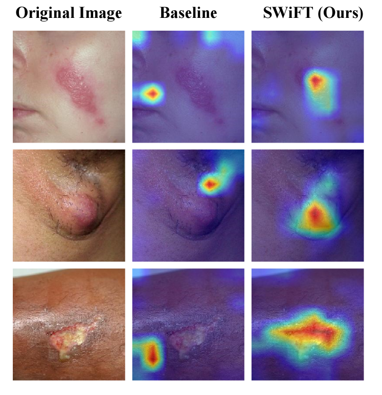
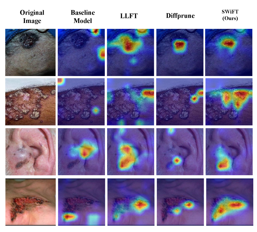
Figure 5 shows exemplary Class Activation Map (CAM) (Zhou et al., 2016) visualizations from the skin classification task. We select images from both the benign and malignant class, as well as different skin attribute groups. The qualitative results in general follow the same behavior of the quantitative results described earlier: Our proposed method provides the best visual results, compared to the best fine-tuning-based method LLFT and the best pruning-based method Diffprune. Specifically, SWiFT successfully redirects attention away from unwanted features, i.e., skin tone, and towards core features, i.e., lesion areas. By constrast, DiffPrune demonstrates smaller activation regions and diminished focus on core features, which indicates that it indiscriminately removes neurons responsible for both bias and core features, leading to loss of information necessary for accurate classification. Although LLFT outperforms the Baseline and DiffPrune with better visual lesion areas, it can still struggle to capture core features when the Baseline model has not learned them robustly. These observations provide clear evidence for the trade-offs detailed in our quantitative results. While prior SOTA methods tend to sacrifice the model’s focus on core features to improve fairness, our method promotes better representation learning and improves overall performance.

5.1.3 Extension to multiple attributes

In the previous sections, we assumed that the sensitive attribute is binary. Towards exploring realistic settings, with more complex fairness-related issues, we further discuss the generalization of our method to multi-attribute scenarios. We consider a problem framing that allows us to reduce the multi-attribute problem to multiple instances of binary-attribute debiasing. It has been previously observed that solely optimizing for worst-group performance can effectively address distribution shifts and mitigate sub-group performance disparities (Sagawa et al., 2019; Liu et al., 2021). We therefore focus on optimizing the worst group via guidance from the best group. Specifically, we reduce the problem to a binary attribute task through selection of the best and worst groups, as defined by AUC, and use the samples from these two groups for optimization. We validate the multi-attribute generalization ability of our method on six skin tone groups and five age groups. As Table 5 shows, our method is consistently effective in both overall AUC, the worst-group AUC, and the AUC gap between the best and the worst group.

Table 5: Comparison of performance of non-binary attributes of skin tone for the skin lesion classification task and age for the chest X-ray classification task. ResNet-50 backbone.

Attr.MethodsFitzpatrick-17k Overall AUC $\uparrow$ Min. AUC $\uparrow$ Gap. AUC $\downarrow$ Skin ToneBaseline0.586 $\pm$ 0.0080.589 $\pm$ 0.0070.048 $\pm$ 0.010SWiFT (Ours)0.599 $\pm$ 0.0250.596 $\pm$ 0.0210.030 $\pm$ 0.005Chexpert Overall AUC $\uparrow$ Min. AUC $\uparrow$ Gap. AUC $\downarrow$ AgeBaseline0.871 $\pm$ 0.0050.813 $\pm$ 0.0050.072 $\pm$ 0.007SWiFT (Ours)0.880 $\pm$ 0.0010.825 $\pm$ 0.0020.068 $\pm$ 0.004

5.2 Ablation Study

We conduct ablative studies on both skin lesion and chest X-ray classification tasks to evaluate the effectiveness of SWiFT in key aspects pertaining to soft-mask utility, efficacy of our fine-tuning components, and the adaptability to external dataset sizes. To this end, we investigate: 1) soft-mask performance compared to the random-mask and hard-mask strategies, and 2) how each step of our fine-tuning process individually impacts fairness and discriminative performance, and 3) performance sensitivity to different sizes of the external dataset.

5.2.1 Sensitivity to masking strategy

We use a soft-mask to preserve discriminative capability while performing debiasing. To evaluate efficacy, we performed a sensitivity study comparing our soft-mask with both a random and a hard-mask. A random soft-mask assigns values by randomly sampling from the $[0,1]$ range. A hard-mask converts the importance scores into binary values based on a predefined threshold. Parameters with importance scores above the threshold are adjusted, while others remain fixed. We search for the optimal fine-tuning rates in $\{0.1,0.3,0.5,0.7,0.9\}$ . The results of the ablation experiments are shown in Table 6. Both soft- and hard-mask strategies outperform random-mask, illustrating the effectiveness of our mask generation process. Moreover, hard-mask performs worse than soft-mask with higher SPD, EOdds and much lower AUC. This shows the difficulty of finding optimal binary mask thresholds. Soft-masking proves to be more flexible and effective in achieving improved fairness-prediction trade-offs.

Table 6: Comparison of random, hard-masks and our proposed mask generation method on skin and gender attributes for the skin lesion classification task. ResNet-50 backbone.

Attr.MethodsFitzpatrick-17k AUC $\uparrow$ SPD $\downarrow$ EOdds $\downarrow$ Skin ToneRandom0.615 $\pm$ 0.0120.119 $\pm$ 0.0160.128 $\pm$ 0.011hard-mask0.622 $\pm$ 0.0020.099 $\pm$ 0.0170.102 $\pm$ 0.017SWiFT (Ours)0.668 $\pm$ 0.0130.092 $\pm$ 0.0280.096 $\pm$ 0.026Atlas AUC $\uparrow$ SPD $\downarrow$ EOdds $\downarrow$ GenderRandom0.787 $\pm$ 0.0040.017 $\pm$ 0.0090.017 $\pm$ 0.008hard-mask0.788 $\pm$ 0.0040.023 $\pm$ 0.0130.023 $\pm$ 0.006SWiFT (Ours)0.789 $\pm$ 0.0050.012 $\pm$ 0.0070.010 $\pm$ 0.006

5.2.2 Sensitivity to mask normalization strategy

Table 7: Comparison of random, hard-masks and our proposed mask generation method on skin and gender attributes for the skin lesion classification task. ResNet-50 backbone.

Attr.MethodsFitzpatrick-17k AUC $\uparrow$ SPD $\downarrow$ EOdds $\downarrow$ Skin Tonez-score0.655 $\pm$ 0.0120.109 $\pm$ 0.0110.105 $\pm$ 0.009SWiFT (Min–Max)0.668 $\pm$ 0.0130.092 $\pm$ 0.0280.096 $\pm$ 0.026Chexpert AUC $\uparrow$ SPD $\downarrow$ EOdds $\downarrow$ Agez-score0.880 $\pm$ 0.0050.087 $\pm$ 0.0280.040 $\pm$ 0.007SWiFT (Min–Max)0.873 $\pm$ 0.0030.059 $\pm$ 0.0190.025 $\pm$ 0.008

For our soft-mask construction, we employ Min-Max normalization over the commonly used z-score method. As shown in Table 7, Min–Max normalization yields superior performance in both AUC and fairness metrics. We attribute this improvement to our mask’s objective: determining the relative ratio between parameter importance for bias and for prediction. Min-Max normalization preserves the shape and relative relationships of the original parameter importance distribution (Singh and Singh, 2020). In contrast, z-score normalization, which re-centers and rescales the data, can distort these crucial relationships. Recognizing that Min-Max normalization is sensitive to outliers, we will explore alternative strategies, such as percentile-based normalization, in future work.

5.2.3 Effectiveness of two-step combination

SWiFT consists of two core steps that contribute to its performance: mask fine-tuning of the feature extractor and partial re-initialization followed by full classification head fine-tuning. To assess the impact of each step, we conducted an ablation study where we compare performance of (i) feature extractor fine-tuning only, (ii) classification head re-initialization and fine-tuning only and (iii) the full pipeline. The results, shown in Table 8, indicate a significant performance decline when either step is removed. However, each individual step still outperforms the Baseline, supporting our hypothesis that bias originates from both feature extraction and feature combination. The integration of both steps effectively eliminates bias from these two sources, resulting in superior performance in terms of both prediction accuracy and fairness.

Table 8: Comparison of performance when ablating fine-tuning components for both skin tone and gender attributes under the skin lesion classification task. ResNet-50 backbone.

Attr.MethodsFitzpatrick-17k AUC $\uparrow$ SPD $\downarrow$ EOdds $\downarrow$ Skin ToneSWiFT (w/o 2nd step)0.605 $\pm$ 0.0090.125 $\pm$ 0.0110.125 $\pm$ 0.010SWiFT (w/o 1st step)0.586 $\pm$ 0.0050.146 $\pm$ 0.0090.146 $\pm$ 0.007SWiFT (Ours)0.668 $\pm$ 0.0130.092 $\pm$ 0.0280.096 $\pm$ 0.026Atlas AUC $\uparrow$ SPD $\downarrow$ EOdds $\downarrow$ GenderSWiFT (w/o 2nd step)0.787 $\pm$ 0.0070.025 $\pm$ 0.0090.021 $\pm$ 0.015SWiFT (w/o 1st step)0.788 $\pm$ 0.0050.022 $\pm$ 0.0070.019 $\pm$ 0.014SWiFT (Ours)0.789 $\pm$ 0.0050.012 $\pm$ 0.0070.010 $\pm$ 0.006

5.2.4 Re-initialization effectiveness

To evaluate the effectiveness of our partial re-initialization strategy, we compare SWiFT with two re-initialization variants, i.e., no classification head re-initialization, and full classification head re-initialization. The results are shown in Table 9. As we can see, both full and partial re-initialization achieve higher accuracy and fairness than the no re-initialization approach, indicating that parameter re-initialization can effectively remove bias and recombine core predictive features. However, partial re-initialization achieves even better results, particularly in terms of AUC. This finding suggests that resetting all parameters in the classification head may lead to catastrophic forgetting of previously learned representations, which complicates the optimization process and ultimately results in suboptimal performance. In contrast, partial re-initialization preserves parameters, important for core features, thus providing favorable seeding for fast and effective fine-tuning.

Table 9: Comparison of performance of partial re-initialization vs full re-initialization strategies of skin tone for the skin lesion classification task and age for the chest X-ray classification task. ResNet-50 backbone.

Attr.MethodsFitzpatrick-17k AUC $\uparrow$ SPD $\downarrow$ EOdds $\downarrow$ Skin ToneNo Reinit0.608 $\pm$ 0.0190.112 $\pm$ 0.0190.103 $\pm$ 0.019Full Reinit0.619 $\pm$ 0.0160.109 $\pm$ 0.0240.105 $\pm$ 0.015SWiFT (Partial)0.668 $\pm$ 0.0130.092 $\pm$ 0.0280.096 $\pm$ 0.026Chexpert AUC $\uparrow$ SPD $\downarrow$ EOdds $\downarrow$ AgeNo Reinit0.873 $\pm$ 0.0040.104 $\pm$ 0.0220.044 $\pm$ 0.008Full Reinit0.876 $\pm$ 0.0040.106 $\pm$ 0.0170.043 $\pm$ 0.007SWiFT (Partial)0.873 $\pm$ 0.0030.059 $\pm$ 0.0190.025 $\pm$ 0.008

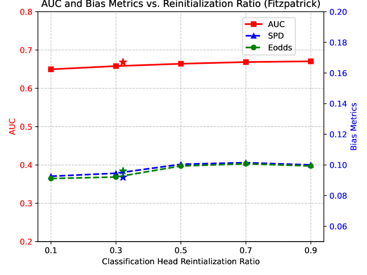
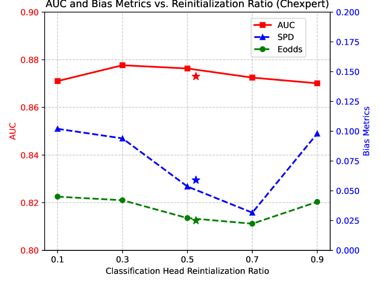
5.2.5 Ablation on the Re-initialization Threshold

We investigate the sensitivity of varying our classification head re-initialization threshold, $\gamma$ . Our analysis compares our proposed heuristic (i.e., setting $\gamma$ to the mean of the mask) against a range of thresholds defined by quantiles of the mask distribution. This corresponds to re-initializing a varying proportion (from 10% to 90%) of classification head parameters with the highest soft-mask values. As shown in Figure 6, the optimal re-initialization ratio is task-dependent and varies across the Fitzpatrick-17k and CheXpert datasets. Notably, our proposed method of setting $\gamma$ to the mean value of the soft-mask calculated on the classification head parameters consistently yields near-optimal prediction and fairness performance without requiring an exhaustive parameter search. This demonstrates that using the mean mask value is a sufficiently effective choice.

5.2.6 Ablation on the Number of Samples

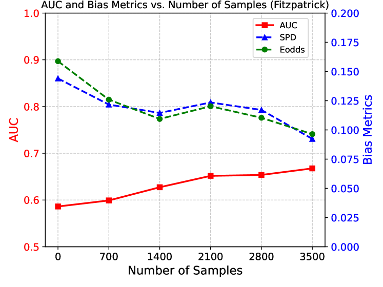
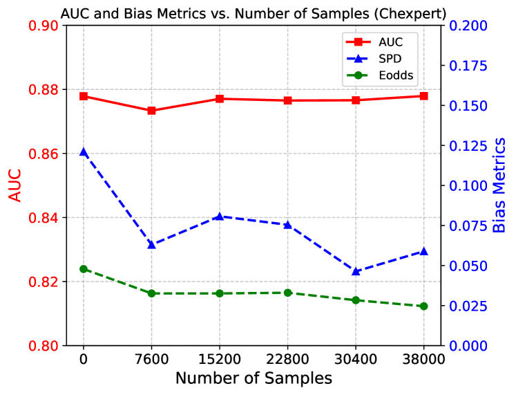
Figure 7 demonstrates the sensitivity of SWiFT performance w.r.t. number of samples on the external dataset. We conducted experiments using $\{0,0.2,0.4,0.6,0.8,1\}$ proportions of the full external dataset, where the 0- sample condition corresponds to the pre-trained Baseline model. As the number of samples increases, the AUC improves while bias decreases. For skin tone, the AUC and bias reach stable after the dataset exceeds 0.4 of its total size (i.e., 1400 samples). Notably, even with a very small external dataset (i.e., $20\%$ of the dataset with 700 samples), SWiFT outperforms the Baseline in both accuracy and fairness. A similar trend emerges in age debiasing on Chexpert, where only $20\%$ of the validation dataset provides a significant improvement in fairness with minimal impact on AUC. The relatively modest increases in AUC across different sample sizes on CheXpert may stem from the already high baseline performance of the pre-trained model, leaving limited room for further improvement. Overall, these findings suggest that SWiFT can operate effectively with relatively small external datasets, highlighting its ease of construction and promising potential for practical advantages in real-world clinical deployments.

5.3 Soft-mask Visualizations and Interpretations

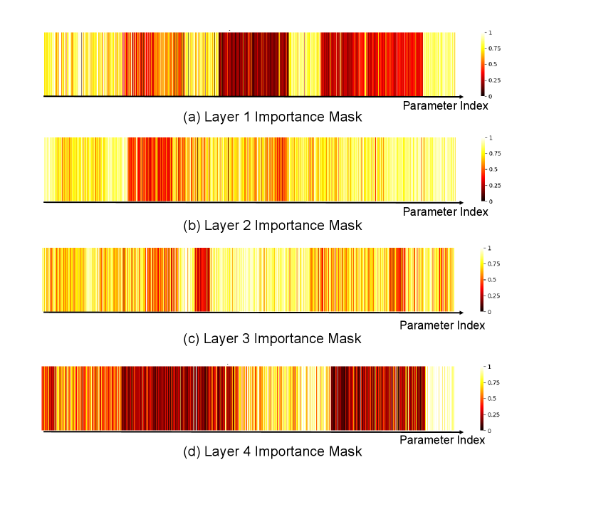
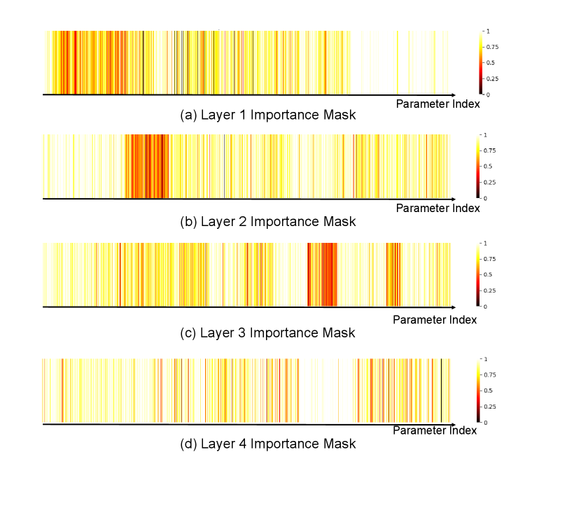
We analyze the distribution of our soft-mask across the layers (residual block group) of a ResNet-50 model to understand how our method allocates parameter updates to address bias and improve core feature learning. Our findings reveal that our mask adaptively identifies different sources of bias depending on the task and model’s initial state.

For the skin tone debiasing task on the ISIC dataset (Figure. 8), the highest mask values are concentrated in the early-to-middle layers (e.g., Layer 2 and Layer 3). This suggests that the updates address the low-level features associated with skin tone bias. Moreover, as the pre-trained has a suboptimal initial AUC, updating shallow layers also improves core representations for better prediction accuracy. In contrast, for the age debiasing task on the MIMIC dataset (Figure. 9), where the model already has a high initial AUC, the mask correctly focuses updates on the deeper layers (e.g., Layer 4). Since the model’s core representations are well-learned, our mask targets the high-level semantic features encoded in deeper layers, which are more likely to be entangled with the abstract concept of age.

6 Limitations and Future Work

Our study has several limitations. First, our experiments were conducted primarily on binary classification tasks with binary sensitive attributes. Although our ablation study provides initial evidence that our method can extend to multi-attribute settings, a comprehensive evaluation on more complex multi-class classification problems is a key next step. However, the core mechanism of our method—disentangling parameter updates based on their importance to task performance versus fairness — is conceptually general. This framework is not intrinsically tied to any specific accuracy or fairness function; therefore, we believe our method can be extended to deal with more diverse prediction or bias settings. Second, our current implementation uses a fixed soft-mask, which is computed once before fine-tuning. This design is based on the assumption that, given the small number of fine-tuning epochs, the relative importance of parameters remains largely stable. This avoids the computational overhead of repeatedly recomputing the mask. However, exploring an adaptive masking strategy, where the mask is updated dynamically, remains a promising direction for future work, especially for applications require longer fine-tuning. Third, while setting the classification head re-initialization threshold to the mean mask value proves to be an effective strategy, future work could explore methods for learning this threshold adaptively. An adaptive threshold may provide a more fine-grained and performant approach to re-initialization.

7 Conclusion

Our study advances bias mitigation in discriminative models trained on dermatological and chest X-ray data. Our method distinguishes core features from biased features, towards enhancing fairness without sacrificing classification performance. Our two-step fine-tuning approach reduces bias under small epoch counts ( ${\sim}10\%$ of original training compute), while remaining agnostic to the choice of model architecture. We thus present an efficient solution, applicable in resource limited scenarios. The challenge of obtaining diverse datasets with comprehensive metadata and sensitive attributes remains a limitation. However, unlike other methods, our approach requires only a small dataset for debiasing, partially alleviating this factor.

Acknowledgments

The work of Junyu Yan was supported in part by the Advanced Care Research Center by the Ph.D. studentship. Sotirios A. Tsaftaris acknowledges support from the Royal Academy of Engineering and the Research Chairs and Senior Research Fellowships scheme (grant RCSRF1819\8\25), and the UK Engineering and Physical Sciences Research Council (EPSRC) support via grant EP/X017680/1, and the UKRI AI programme, for the Causality in Healthcare AI Hub (CHAI, grant EP/Y028856/1).

Ethical Standards

The work follows appropriate ethical standards in conducting research and writing the manuscript, following all applicable laws and regulations regarding treatment of animals or human subjects.

Conflicts of Interest

We declare we don’t have conflicts of interest.

Data availability

All data used in the experiments is publicly available. The ISIC dataset, Fitzpatrick-17k dataset, and Atlas dataset can be obtained based on instructions at https://github.com/pbevan1/Skin-Deep-Unlearning. The provided codebase contains implementation for all additional data pre-processing that was done. The DDI dataset can be accessed at https://ddi-dataset.github.io/. The PAD-UFES-20 dataset can be accessed at https://data.mendeley.com/datasets/zr7vgbcyr2/1. The MIMIC dataset can be downloaded from https://physionet.org/content/mimic-cxr/2.1.0/. The Chexpert dataset can be accessed at https://stanfordmlgroup.github.io/competitions/chexpert/. The NIH dataset can be accessed at https://www.kaggle.com/datasets/nih-chest-xrays/data

References

Ben Zaken et al. (2022) Elad Ben Zaken, Yoav Goldberg, and Shauli Ravfogel. BitFit: Simple parameter-efficient fine-tuning for transformer-based masked language-models. In Proceedings of the 60th Annual Meeting of the Association for Computational Linguistics (Volume 2: Short Papers). Association for Computational Linguistics, May 2022.
Bevan and Atapour-Abarghouei (2022) Peter Bevan and Amir Atapour-Abarghouei. Skin deep unlearning: Artefact and instrument debiasing in the context of melanoma classification. In International Conference on Machine Learning, pages 1874–1892. PMLR, 2022.
Bissoto et al. (2020) Alceu Bissoto, Eduardo Valle, and Sandra Avila. Debiasing skin lesion datasets and models? not so fast. In Proceedings of the IEEE/CVF Conference on Computer Vision and Pattern Recognition Workshops, pages 740–741, 2020.
Chen et al. (2024) Ruizhe Chen, Jianfei Yang, Huimin Xiong, Jianhong Bai, Tianxiang Hu, Jin Hao, Yang Feng, Joey Tianyi Zhou, Jian Wu, and Zuozhu Liu. Fast model debias with machine unlearning. Advances in Neural Information Processing Systems, 36, 2024.
Cherepanova et al. (2021) Valeriia Cherepanova, Vedant Nanda, Micah Goldblum, John P Dickerson, and Tom Goldstein. Technical challenges for training fair neural networks. arXiv preprint arXiv:2102.06764, 2021.
Codella et al. (2019) Noel Codella, Veronica Rotemberg, Philipp Tschandl, M Emre Celebi, et al. Skin lesion analysis toward melanoma detection 2018: A challenge hosted by the international skin imaging collaboration (ISIC). arXiv preprint arXiv:1902.03368, 2019.
Codella et al. (2018) Noel CF Codella, David Gutman, M Emre Celebi, Brian Helba, Michael A Marchetti, Stephen W Dusza, Aadi Kalloo, et al. Skin lesion analysis toward melanoma detection: A challenge at the 2017 international symposium on biomedical imaging (ISBI), hosted by the international skin imaging collaboration (ISIC). In 2018 IEEE 15th international symposium on biomedical imaging (ISBI 2018), pages 168–172. IEEE, 2018.
Daneshjou et al. (2022) Roxana Daneshjou, Kailas Vodrahalli, Roberto A Novoa, Melissa Jenkins, Weixin Liang, Veronica Rotemberg, Justin Ko, Susan M Swetter, et al. Disparities in dermatology ai performance on a diverse, curated clinical image set. Science advances, 8(31):6147, 2022.
Dutt et al. (2024) Raman Dutt, Ondrej Bohdal, Sotirios A Tsaftaris, and Timothy Hospedales. Fairtune: Optimizing parameter efficient fine tuning for fairness in medical image analysis. In The Twelfth International Conference on Learning Representations, 2024.
Dwork et al. (2012) Cynthia Dwork, Moritz Hardt, Toniann Pitassi, Omer Reingold, and Richard Zemel. Fairness through awareness. In Proceedings of the 3rd Innovations in Theoretical Computer Science Conference, pages 214–226, 2012.
Foster et al. (2024) Jack Foster, Stefan Schoepf, and Alexandra Brintrup. Fast machine unlearning without retraining through selective synaptic dampening. In Proceedings of the AAAI Conference on Artificial Intelligence, volume 38, pages 12043–12051, 2024.
Groh et al. (2021) Matthew Groh, Caleb Harris, Luis Soenksen, Felix Lau, Rachel Han, Aerin Kim, Arash Koochek, and Omar Badri. Evaluating deep neural networks trained on clinical images in dermatology with the fitzpatrick 17k dataset. In Proceedings of the IEEE/CVF Conference on Computer Vision and Pattern Recognition, pages 1820–1828, 2021.
Hardt et al. (2016) Moritz Hardt, Eric Price, and Nati Srebro. Equality of opportunity in supervised learning. Advances in Neural Information Processing Systems, 29, 2016.
Hendrycks et al. (2019) Dan Hendrycks, Kimin Lee, and Mantas Mazeika. Using pre-training can improve model robustness and uncertainty. In International conference on machine learning, pages 2712–2721. PMLR, 2019.
Hernández-Pérez et al. (2024) Carlos Hernández-Pérez, Marc Combalia, Sebastian Podlipnik, Noel CF Codella, Veronica Rotemberg, Allan C Halpern, Ofer Reiter, Cristina Carrera, Alicia Barreiro, Brian Helba, et al. Bcn20000: Dermoscopic lesions in the wild. Scientific Data, 11(1):641, 2024.
Irvin et al. (2019) Jeremy Irvin, Pranav Rajpurkar, Michael Ko, Yifan Yu, Silviana Ciurea-Ilcus, Chris Chute, Henrik Marklund, Behzad Haghgoo, Robyn Ball, Katie Shpanskaya, et al. Chexpert: A large chest radiograph dataset with uncertainty labels and expert comparison. In Proceedings of the AAAI conference on artificial intelligence, volume 33, pages 590–597, 2019.
Johnson et al. (2019) Alistair EW Johnson, Tom J Pollard, Nathaniel R Greenbaum, Matthew P Lungren, Chih-ying Deng, Yifan Peng, Zhiyong Lu, Roger G Mark, Seth J Berkowitz, and Steven Horng. Mimic-cxr-jpg, a large publicly available database of labeled chest radiographs. arXiv preprint arXiv:1901.07042, 2019.
Jung et al. (2023) Sangwon Jung, Taeeon Park, Sanghyuk Chun, and Taesup Moon. Re-weighting based group fairness regularization via classwise robust optimization. In 11th International Conference on Learning Representations, ICLR 2023, 2023.
Kirichenko et al. (2023) Polina Kirichenko, Pavel Izmailov, and Andrew Gordon Wilson. Last layer re-training is sufficient for robustness to spurious correlations. In The Eleventh International Conference on Learning Representations, 2023.
Kirkpatrick et al. (2017) James Kirkpatrick, Razvan Pascanu, Neil Rabinowitz, Joel Veness, Guillaume Desjardins, Andrei A Rusu, Kieran Milan, John Quan, Tiago Ramalho, Agnieszka Grabska-Barwinska, et al. Overcoming catastrophic forgetting in neural networks. Proceedings of the national academy of sciences, 114(13):3521–3526, 2017.
Konishi et al. (2023) Tatsuya Konishi, Mori Kurokawa, Chihiro Ono, Zixuan Ke, Gyuhak Kim, and Bing Liu. Parameter-level soft-masking for continual learning. In International Conference on Machine Learning, pages 17492–17505. PMLR, 2023.
Le et al. (2023) Phuong Quynh Le, Jörg Schlötterer, and Christin Seifert. Is last layer re-training truly sufficient for robustness to spurious correlations? arXiv preprint arXiv:2308.00473, 2023.
Li et al. (2020) Xingjian Li, Haoyi Xiong, Haozhe An, Cheng-Zhong Xu, and Dejing Dou. Rifle: Backpropagation in depth for deep transfer learning through re-initializing the fully-connected layer. In International Conference on Machine Learning, pages 6010–6019. PMLR, 2020.
Lio and Nghiem (2004) Peter A Lio and Paul Nghiem. Interactive atlas of dermoscopy. Journal of the American Academy of Dermatology, 50(5):807–808, 2004.
Liu et al. (2021) Evan Z Liu, Behzad Haghgoo, Annie S Chen, Aditi Raghunathan, Pang Wei Koh, Shiori Sagawa, Percy Liang, and Chelsea Finn. Just train twice: Improving group robustness without training group information. In International Conference on Machine Learning, pages 6781–6792. PMLR, 2021.
Luo et al. (2024) Yan Luo, Yu Tian, Min Shi, Louis R Pasquale, Lucy Q Shen, Nazlee Zebardast, Tobias Elze, and Mengyu Wang. Harvard glaucoma fairness: a retinal nerve disease dataset for fairness learning and fair identity normalization. IEEE Transactions on Medical Imaging, 2024.
Mao et al. (2023) Yuzhen Mao, Zhun Deng, Huaxiu Yao, Kenji Kawaguchi, and James Zou. Last-layer fairness fine-tuning is simple and effective for neural networks. In ICML 2023 Workshop on Spurious Correlations, Invariance, and Stability, 2023.
Marcinkevics et al. (2022) Ricards Marcinkevics, Ece Ozkan, and Julia E Vogt. Debiasing deep chest x-ray classifiers using intra-and post-processing methods. In Machine Learning for Healthcare Conference, pages 504–536. PMLR, 2022.
Mehrabi et al. (2021) Ninareh Mehrabi, Fred Morstatter, Nripsuta Saxena, Kristina Lerman, and Aram Galstyan. A survey on bias and fairness in machine learning. ACM computing surveys (CSUR), 54(6):1–35, 2021.
Oguguo et al. (2023) Tochi Oguguo, Ghada Zamzmi, Sivaramakrishnan Rajaraman, Feng Yang, Zhiyun Xue, and Sameer Antani. A comparative study of fairness in medical machine learning. In 2023 IEEE 20th International Symposium on Biomedical Imaging (ISBI), pages 1–5. IEEE, 2023.
Pacheco et al. (2020) Andre GC Pacheco, Gustavo R Lima, Amanda S Salomao, Breno Krohling, Igor P Biral, Gabriel G de Angelo, et al. Pad-ufes-20: A skin lesion dataset composed of patient data and clinical images collected from smartphones. Data in Brief, 32:106221, 2020.
Park et al. (2022) Sungho Park, Jewook Lee, Pilhyeon Lee, Sunhee Hwang, Dohyung Kim, and Hyeran Byun. Fair contrastive learning for facial attribute classification. In Proceedings of the IEEE/CVF Conference on Computer Vision and Pattern Recognition, pages 10389–10398, 2022.
Puyol-Antón et al. (2021) Esther Puyol-Antón, Bram Ruijsink, Stefan K Piechnik, Stefan Neubauer, et al. Fairness in cardiac MR image analysis: an investigation of bias due to data imbalance in deep learning based segmentation. In Medical Image Computing and Computer Assisted Intervention–MICCAI 2021, September 27–October 1, 2021, Proceedings, Part III 24, pages 413–423. Springer, 2021.
Ramkumar et al. (2024) Vijaya Raghavan T Ramkumar, Bahram Zonooz, and Elahe Arani. The effectiveness of random forgetting for robust generalization. In The Twelfth International Conference on Learning Representations, 2024.
Rotemberg et al. (2021) Veronica Rotemberg, Nicholas Kurtansky, Brigid Betz-Stablein, Liam Caffery, Emmanouil Chousakos, Noel Codella, et al. A patient-centric dataset of images and metadata for identifying melanomas using clinical context. Scientific data, 8(1):34, 2021.
Sagawa et al. (2019) Shiori Sagawa, Pang Wei Koh, Tatsunori B Hashimoto, and Percy Liang. Distributionally robust neural networks for group shifts: On the importance of regularization for worst-case generalization. arXiv preprint arXiv:1911.08731, 2019.
Seyyed-Kalantari et al. (2020) Laleh Seyyed-Kalantari, Guanxiong Liu, Matthew McDermott, Irene Y Chen, and Marzyeh Ghassemi. Chexclusion: Fairness gaps in deep chest x-ray classifiers. In BIOCOMPUTING 2021: proceedings of the Pacific symposium, pages 232–243. World Scientific, 2020.
Singh and Singh (2020) Dalwinder Singh and Birmohan Singh. Investigating the impact of data normalization on classification performance. Applied Soft Computing, 97:105524, 2020.
Singh and Bajorek (2014) Shamsher Singh and Beata Bajorek. Defining ‘elderly’in clinical practice guidelines for pharmacotherapy. Pharmacy practice, 12(4), 2014.
Tschandl et al. (2018) Philipp Tschandl, Cliff Rosendahl, and Harald Kittler. The HAM10000 dataset, a large collection of multi-source dermatoscopic images of common pigmented skin lesions. Scientific data, 5(1):1–9, 2018.
Wang et al. (2017) Xiaosong Wang, Yifan Peng, Le Lu, Zhiyong Lu, Mohammadhadi Bagheri, and Ronald M Summers. Chestx-ray8: Hospital-scale chest x-ray database and benchmarks on weakly-supervised classification and localization of common thorax diseases. In Proceedings of the IEEE conference on computer vision and pattern recognition, pages 2097–2106, 2017.
Wu et al. (2022) Yawen Wu, Dewen Zeng, Xiaowei Xu, and Jingtong Hu. FairPrune: Achieving fairness through pruning for dermatological disease diagnosis. In International Conference on Medical Image Computing and Computer-Assisted Intervention, pages 743–753. Springer, 2022.
Xu et al. (2023) Zikang Xu, Jun Li, Qingsong Yao, Han Li, and S Kevin Zhou. Fairness in medical image analysis and healthcare: A literature survey. Authorea Preprints, 2023.
Xue et al. (2024) Yuyang Xue, Junyu Yan, Raman Dutt, Fasih Haider, Jingshuai Liu, Steven McDonagh, and Sotirios A Tsaftaris. Bmft: Achieving fairness via bias-based weight masking fine-tuning. In MICCAI Workshop on Fairness of AI in Medical Imaging, 2024.
Yuan et al. (2019) Changan Yuan, Yong Wu, Xiao Qin, Shaojie Qiao, Yonghua Pan, Ping Huang, Dunhu Liu, and Nan Han. An effective image classification method for shallow densely connected convolution networks through squeezing and splitting techniques. Applied Intelligence, 49:3570–3586, 2019.
Yuan et al. (2023) Haolin Yuan, John Aucott, Armin Hadzic, William Paul, Marcia Villegas de Flores, Philip Mathew, Philippe Burlina, and Yinzhi Cao. Edgemixup: embarrassingly simple data alteration to improve lyme disease lesion segmentation and diagnosis fairness. In International Conference on Medical Image Computing and Computer-Assisted Intervention, pages 374–384. Springer, 2023.
Zafar et al. (2017) Muhammad Bilal Zafar, Isabel Valera, Manuel Gomez Rogriguez, and Krishna P Gummadi. Fairness constraints: Mechanisms for fair classification. In Artificial intelligence and statistics, pages 962–970. PMLR, 2017.
Zhang et al. (2017) Chen-Lin Zhang, Jian-Hao Luo, Xiu-Shen Wei, and Jianxin Wu. In defense of fully connected layers in visual representation transfer. In Pacific Rim Conference on Multimedia, pages 807–817. Springer, 2017.
Zhang et al. (2022) Haoran Zhang, Natalie Dullerud, Karsten Roth, Lauren Oakden-Rayner, Stephen Pfohl, and Marzyeh Ghassemi. Improving the fairness of chest x-ray classifiers. In Conference on health, inference, and learning, pages 204–233. PMLR, 2022.
Zhao et al. (2022) Jiawei Zhao, Florian Tobias Schaefer, and Anima Anandkumar. Zero initialization: Initializing neural networks with only zeros and ones. Transactions on Machine Learning Research, 2022.
Zhou et al. (2016) Bolei Zhou, Aditya Khosla, Agata Lapedriza, Aude Oliva, and Antonio Torralba. Learning deep features for discriminative localization. In Proceedings of the IEEE conference on computer vision and pattern recognition, pages 2921–2929, 2016.
Zietlow et al. (2022) Dominik Zietlow, Michael Lohaus, Guha Balakrishnan, Matthaeus Kleindessner, Francesco Locatello, B Scholkopf, and Chris Russell. Leveling down in computer vision: Pareto inefficiencies in fair deep classifiers. in 2022 ieee. In CVF Conference on Computer Vision and Pattern Recognition (CVPR), pages 10400–10411, 2022.

[bib.bib1] Ben Zaken et al. (2022) Elad Ben Zaken, Yoav Goldberg, and Shauli Ravfogel. BitFit: Simple parameter-efficient fine-tuning for transformer-based masked language-models. In Proceedings of the 60th Annual Meeting of the Association for Computational Linguistics (Volume 2: Short Papers). Association for Computational Linguistics, May 2022.

[bib.bib2] Bevan and Atapour-Abarghouei (2022) Peter Bevan and Amir Atapour-Abarghouei. Skin deep unlearning: Artefact and instrument debiasing in the context of melanoma classification. In International Conference on Machine Learning, pages 1874–1892. PMLR, 2022.

[bib.bib3] Bissoto et al. (2020) Alceu Bissoto, Eduardo Valle, and Sandra Avila. Debiasing skin lesion datasets and models? not so fast. In Proceedings of the IEEE/CVF Conference on Computer Vision and Pattern Recognition Workshops, pages 740–741, 2020.

[bib.bib4] Chen et al. (2024) Ruizhe Chen, Jianfei Yang, Huimin Xiong, Jianhong Bai, Tianxiang Hu, Jin Hao, Yang Feng, Joey Tianyi Zhou, Jian Wu, and Zuozhu Liu. Fast model debias with machine unlearning. Advances in Neural Information Processing Systems, 36, 2024.

[bib.bib5] Cherepanova et al. (2021) Valeriia Cherepanova, Vedant Nanda, Micah Goldblum, John P Dickerson, and Tom Goldstein. Technical challenges for training fair neural networks. arXiv preprint arXiv:2102.06764, 2021.

[bib.bib6] Codella et al. (2019) Noel Codella, Veronica Rotemberg, Philipp Tschandl, M Emre Celebi, et al. Skin lesion analysis toward melanoma detection 2018: A challenge hosted by the international skin imaging collaboration (ISIC). arXiv preprint arXiv:1902.03368, 2019.

[bib.bib7] Codella et al. (2018) Noel CF Codella, David Gutman, M Emre Celebi, Brian Helba, Michael A Marchetti, Stephen W Dusza, Aadi Kalloo, et al. Skin lesion analysis toward melanoma detection: A challenge at the 2017 international symposium on biomedical imaging (ISBI), hosted by the international skin imaging collaboration (ISIC). In 2018 IEEE 15th international symposium on biomedical imaging (ISBI 2018), pages 168–172. IEEE, 2018.

[bib.bib8] Daneshjou et al. (2022) Roxana Daneshjou, Kailas Vodrahalli, Roberto A Novoa, Melissa Jenkins, Weixin Liang, Veronica Rotemberg, Justin Ko, Susan M Swetter, et al. Disparities in dermatology ai performance on a diverse, curated clinical image set. Science advances, 8(31):6147, 2022.

[bib.bib9] Dutt et al. (2024) Raman Dutt, Ondrej Bohdal, Sotirios A Tsaftaris, and Timothy Hospedales. Fairtune: Optimizing parameter efficient fine tuning for fairness in medical image analysis. In The Twelfth International Conference on Learning Representations, 2024.

[bib.bib10] Dwork et al. (2012) Cynthia Dwork, Moritz Hardt, Toniann Pitassi, Omer Reingold, and Richard Zemel. Fairness through awareness. In Proceedings of the 3rd Innovations in Theoretical Computer Science Conference, pages 214–226, 2012.

[bib.bib11] Foster et al. (2024) Jack Foster, Stefan Schoepf, and Alexandra Brintrup. Fast machine unlearning without retraining through selective synaptic dampening. In Proceedings of the AAAI Conference on Artificial Intelligence, volume 38, pages 12043–12051, 2024.

[bib.bib12] Groh et al. (2021) Matthew Groh, Caleb Harris, Luis Soenksen, Felix Lau, Rachel Han, Aerin Kim, Arash Koochek, and Omar Badri. Evaluating deep neural networks trained on clinical images in dermatology with the fitzpatrick 17k dataset. In Proceedings of the IEEE/CVF Conference on Computer Vision and Pattern Recognition, pages 1820–1828, 2021.

[bib.bib13] Hardt et al. (2016) Moritz Hardt, Eric Price, and Nati Srebro. Equality of opportunity in supervised learning. Advances in Neural Information Processing Systems, 29, 2016.

[bib.bib14] Hendrycks et al. (2019) Dan Hendrycks, Kimin Lee, and Mantas Mazeika. Using pre-training can improve model robustness and uncertainty. In International conference on machine learning, pages 2712–2721. PMLR, 2019.

[bib.bib15] Hernández-Pérez et al. (2024) Carlos Hernández-Pérez, Marc Combalia, Sebastian Podlipnik, Noel CF Codella, Veronica Rotemberg, Allan C Halpern, Ofer Reiter, Cristina Carrera, Alicia Barreiro, Brian Helba, et al. Bcn20000: Dermoscopic lesions in the wild. Scientific Data, 11(1):641, 2024.

[bib.bib16] Irvin et al. (2019) Jeremy Irvin, Pranav Rajpurkar, Michael Ko, Yifan Yu, Silviana Ciurea-Ilcus, Chris Chute, Henrik Marklund, Behzad Haghgoo, Robyn Ball, Katie Shpanskaya, et al. Chexpert: A large chest radiograph dataset with uncertainty labels and expert comparison. In Proceedings of the AAAI conference on artificial intelligence, volume 33, pages 590–597, 2019.

[bib.bib17] Johnson et al. (2019) Alistair EW Johnson, Tom J Pollard, Nathaniel R Greenbaum, Matthew P Lungren, Chih-ying Deng, Yifan Peng, Zhiyong Lu, Roger G Mark, Seth J Berkowitz, and Steven Horng. Mimic-cxr-jpg, a large publicly available database of labeled chest radiographs. arXiv preprint arXiv:1901.07042, 2019.

[bib.bib18] Jung et al. (2023) Sangwon Jung, Taeeon Park, Sanghyuk Chun, and Taesup Moon. Re-weighting based group fairness regularization via classwise robust optimization. In 11th International Conference on Learning Representations, ICLR 2023, 2023.

[bib.bib19] Kirichenko et al. (2023) Polina Kirichenko, Pavel Izmailov, and Andrew Gordon Wilson. Last layer re-training is sufficient for robustness to spurious correlations. In The Eleventh International Conference on Learning Representations, 2023.

[bib.bib20] Kirkpatrick et al. (2017) James Kirkpatrick, Razvan Pascanu, Neil Rabinowitz, Joel Veness, Guillaume Desjardins, Andrei A Rusu, Kieran Milan, John Quan, Tiago Ramalho, Agnieszka Grabska-Barwinska, et al. Overcoming catastrophic forgetting in neural networks. Proceedings of the national academy of sciences, 114(13):3521–3526, 2017.

[bib.bib21] Konishi et al. (2023) Tatsuya Konishi, Mori Kurokawa, Chihiro Ono, Zixuan Ke, Gyuhak Kim, and Bing Liu. Parameter-level soft-masking for continual learning. In International Conference on Machine Learning, pages 17492–17505. PMLR, 2023.

[bib.bib22] Le et al. (2023) Phuong Quynh Le, Jörg Schlötterer, and Christin Seifert. Is last layer re-training truly sufficient for robustness to spurious correlations? arXiv preprint arXiv:2308.00473, 2023.

[bib.bib23] Li et al. (2020) Xingjian Li, Haoyi Xiong, Haozhe An, Cheng-Zhong Xu, and Dejing Dou. Rifle: Backpropagation in depth for deep transfer learning through re-initializing the fully-connected layer. In International Conference on Machine Learning, pages 6010–6019. PMLR, 2020.

[bib.bib24] Lio and Nghiem (2004) Peter A Lio and Paul Nghiem. Interactive atlas of dermoscopy. Journal of the American Academy of Dermatology, 50(5):807–808, 2004.

[bib.bib25] Liu et al. (2021) Evan Z Liu, Behzad Haghgoo, Annie S Chen, Aditi Raghunathan, Pang Wei Koh, Shiori Sagawa, Percy Liang, and Chelsea Finn. Just train twice: Improving group robustness without training group information. In International Conference on Machine Learning, pages 6781–6792. PMLR, 2021.

[bib.bib26] Luo et al. (2024) Yan Luo, Yu Tian, Min Shi, Louis R Pasquale, Lucy Q Shen, Nazlee Zebardast, Tobias Elze, and Mengyu Wang. Harvard glaucoma fairness: a retinal nerve disease dataset for fairness learning and fair identity normalization. IEEE Transactions on Medical Imaging, 2024.

[bib.bib27] Mao et al. (2023) Yuzhen Mao, Zhun Deng, Huaxiu Yao, Kenji Kawaguchi, and James Zou. Last-layer fairness fine-tuning is simple and effective for neural networks. In ICML 2023 Workshop on Spurious Correlations, Invariance, and Stability, 2023.

[bib.bib28] Marcinkevics et al. (2022) Ricards Marcinkevics, Ece Ozkan, and Julia E Vogt. Debiasing deep chest x-ray classifiers using intra-and post-processing methods. In Machine Learning for Healthcare Conference, pages 504–536. PMLR, 2022.

[bib.bib29] Mehrabi et al. (2021) Ninareh Mehrabi, Fred Morstatter, Nripsuta Saxena, Kristina Lerman, and Aram Galstyan. A survey on bias and fairness in machine learning. ACM computing surveys (CSUR), 54(6):1–35, 2021.

[bib.bib30] Oguguo et al. (2023) Tochi Oguguo, Ghada Zamzmi, Sivaramakrishnan Rajaraman, Feng Yang, Zhiyun Xue, and Sameer Antani. A comparative study of fairness in medical machine learning. In 2023 IEEE 20th International Symposium on Biomedical Imaging (ISBI), pages 1–5. IEEE, 2023.

[bib.bib31] Pacheco et al. (2020) Andre GC Pacheco, Gustavo R Lima, Amanda S Salomao, Breno Krohling, Igor P Biral, Gabriel G de Angelo, et al. Pad-ufes-20: A skin lesion dataset composed of patient data and clinical images collected from smartphones. Data in Brief, 32:106221, 2020.

[bib.bib32] Park et al. (2022) Sungho Park, Jewook Lee, Pilhyeon Lee, Sunhee Hwang, Dohyung Kim, and Hyeran Byun. Fair contrastive learning for facial attribute classification. In Proceedings of the IEEE/CVF Conference on Computer Vision and Pattern Recognition, pages 10389–10398, 2022.

[bib.bib33] Puyol-Antón et al. (2021) Esther Puyol-Antón, Bram Ruijsink, Stefan K Piechnik, Stefan Neubauer, et al. Fairness in cardiac MR image analysis: an investigation of bias due to data imbalance in deep learning based segmentation. In Medical Image Computing and Computer Assisted Intervention–MICCAI 2021, September 27–October 1, 2021, Proceedings, Part III 24, pages 413–423. Springer, 2021.

[bib.bib34] Ramkumar et al. (2024) Vijaya Raghavan T Ramkumar, Bahram Zonooz, and Elahe Arani. The effectiveness of random forgetting for robust generalization. In The Twelfth International Conference on Learning Representations, 2024.

[bib.bib35] Rotemberg et al. (2021) Veronica Rotemberg, Nicholas Kurtansky, Brigid Betz-Stablein, Liam Caffery, Emmanouil Chousakos, Noel Codella, et al. A patient-centric dataset of images and metadata for identifying melanomas using clinical context. Scientific data, 8(1):34, 2021.

[bib.bib36] Sagawa et al. (2019) Shiori Sagawa, Pang Wei Koh, Tatsunori B Hashimoto, and Percy Liang. Distributionally robust neural networks for group shifts: On the importance of regularization for worst-case generalization. arXiv preprint arXiv:1911.08731, 2019.

[bib.bib37] Seyyed-Kalantari et al. (2020) Laleh Seyyed-Kalantari, Guanxiong Liu, Matthew McDermott, Irene Y Chen, and Marzyeh Ghassemi. Chexclusion: Fairness gaps in deep chest x-ray classifiers. In BIOCOMPUTING 2021: proceedings of the Pacific symposium, pages 232–243. World Scientific, 2020.

[bib.bib38] Singh and Singh (2020) Dalwinder Singh and Birmohan Singh. Investigating the impact of data normalization on classification performance. Applied Soft Computing, 97:105524, 2020.

[bib.bib39] Singh and Bajorek (2014) Shamsher Singh and Beata Bajorek. Defining ‘elderly’in clinical practice guidelines for pharmacotherapy. Pharmacy practice, 12(4), 2014.

[bib.bib40] Tschandl et al. (2018) Philipp Tschandl, Cliff Rosendahl, and Harald Kittler. The HAM10000 dataset, a large collection of multi-source dermatoscopic images of common pigmented skin lesions. Scientific data, 5(1):1–9, 2018.

[bib.bib41] Wang et al. (2017) Xiaosong Wang, Yifan Peng, Le Lu, Zhiyong Lu, Mohammadhadi Bagheri, and Ronald M Summers. Chestx-ray8: Hospital-scale chest x-ray database and benchmarks on weakly-supervised classification and localization of common thorax diseases. In Proceedings of the IEEE conference on computer vision and pattern recognition, pages 2097–2106, 2017.

[bib.bib42] Wu et al. (2022) Yawen Wu, Dewen Zeng, Xiaowei Xu, and Jingtong Hu. FairPrune: Achieving fairness through pruning for dermatological disease diagnosis. In International Conference on Medical Image Computing and Computer-Assisted Intervention, pages 743–753. Springer, 2022.

[bib.bib43] Xu et al. (2023) Zikang Xu, Jun Li, Qingsong Yao, Han Li, and S Kevin Zhou. Fairness in medical image analysis and healthcare: A literature survey. Authorea Preprints, 2023.

[bib.bib44] Xue et al. (2024) Yuyang Xue, Junyu Yan, Raman Dutt, Fasih Haider, Jingshuai Liu, Steven McDonagh, and Sotirios A Tsaftaris. Bmft: Achieving fairness via bias-based weight masking fine-tuning. In MICCAI Workshop on Fairness of AI in Medical Imaging, 2024.

[bib.bib45] Yuan et al. (2019) Changan Yuan, Yong Wu, Xiao Qin, Shaojie Qiao, Yonghua Pan, Ping Huang, Dunhu Liu, and Nan Han. An effective image classification method for shallow densely connected convolution networks through squeezing and splitting techniques. Applied Intelligence, 49:3570–3586, 2019.

[bib.bib46] Yuan et al. (2023) Haolin Yuan, John Aucott, Armin Hadzic, William Paul, Marcia Villegas de Flores, Philip Mathew, Philippe Burlina, and Yinzhi Cao. Edgemixup: embarrassingly simple data alteration to improve lyme disease lesion segmentation and diagnosis fairness. In International Conference on Medical Image Computing and Computer-Assisted Intervention, pages 374–384. Springer, 2023.

[bib.bib47] Zafar et al. (2017) Muhammad Bilal Zafar, Isabel Valera, Manuel Gomez Rogriguez, and Krishna P Gummadi. Fairness constraints: Mechanisms for fair classification. In Artificial intelligence and statistics, pages 962–970. PMLR, 2017.